Revised simplex algorithm¶

Part 4 · Matrix methods, sensitivity and geometry · Chapter 11 · Lecture notes, volume 4 (PDF) · Exercises: Revised simplex algorithm

Example 11.1: an LP problem in canonical form and its standard form

We consider the following LP problem in canonical maximization form with \(n=2\) variables and \(m=3\) constraints:

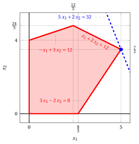
\[ \begin{array}{rrrrrrrrrrrrr} {\max} & 5 \, {x_1} & {+} & 2 \, {x_2} \\[2ex] \text{subject to} & {-} \, {x_1} & {+} & 3 \, {x_2} & {\le} & 12 \\[2ex] & {x_1} & {+} & 2 \, {x_2} & {\le} & 12 \\[2ex] & {3} \, {x_1} & {-} & 2 \, {x_2} & {\le} & {8} \\[2ex] & {x_1,} & & {x_2} & { \ge} & {0} \end{array} \]

Its equivalent standard form with \(n+m=5\) variables and \(m=3\) constraints is:

\[ \begin{array}{rrrrrrrrrrrrrrrrrrr} {\max} & 5 \, {x_1} & {+} & 2 \, {x_2} & & \\[1ex] \text{subject to} & {-x_1} & {+} & {3} \, {x_2} & {+} \, {x_3} & & & {=} & 12 \\[1ex] & {x_1} & {+} & {2} \, {x_2} & & {+} \, {x_4} & & {=} & 12 \\[1ex] & 3 \, {x_1} & {-} & {2} \, {x_2} & & & {+} \, {x_5} & {=} & 8 \\[1ex] & {x_1,} & & {x_2,} & \, {x_3,} & \, {x_4,} & \, {x_5} & { \ge} & { 0 } \end{array} \]

For this LP problem in standard form, we have:

\[ {\boldsymbol c}= \begin{pmatrix} 5 \\[0.5ex] 2 \\[0.5ex] 0 \\[0.5ex] 0 \\[0.5ex] 0 \end{pmatrix} \quad {\boldsymbol x}= \begin{pmatrix} x_{1} \\[0.5ex] x_{2} \\[0.5ex] x_{3} \\[0.5ex] x_{4} \\[0.5ex] x_{5} \end{pmatrix} \quad {\boldsymbol A}= \begin{pmatrix} -1 & 3 & 1 & 0 & 0\\[1ex] 1 & 2 & 0 & 1 & 0\\[1ex] 3 & -2 & 0 & 0 & 1\\ \end{pmatrix} \quad {\boldsymbol b}= \begin{pmatrix} 12 \\[1ex] 12 \\[1ex] 8 \\ \end{pmatrix} \]

Since \(\begin{pmatrix} 12 \\[1ex] 12 \\[1ex] 8 \end{pmatrix} \ge \begin{pmatrix} 0 \\[1ex] 0 \\[1ex] 0 \end{pmatrix}\), with \(\pazocal{B}=\{3,4,5\}\) and \(\pazocal{N}=\{1,2\}\) we have the following initial basic feasible solution:

\[ \begin{pmatrix} x_3 \\[1ex] x_4 \\[1ex] x_5 \\ \end{pmatrix} = \begin{pmatrix} 12 \\[1ex] 12 \\[1ex] 8 \\ \end{pmatrix} ~~~~~ \begin{pmatrix} x_1 \\[1ex] x_2 \end{pmatrix} = \begin{pmatrix} 0 \\[1ex] 0 \end{pmatrix} \text{ and } \bar{\boldsymbol b}= \begin{pmatrix} 12\\[1ex] 12\\[1ex] 8 \end{pmatrix} \]

11.1 Pivoting operations with two systems of linear equations¶

Given a basis \({\boldsymbol A}_{\pazocal{B}}\), all the information necessary for the pivoting operations can be determined by solving two systems of linear equations.
1. First system of linear equations
- The reduced costs and the basic feasible solution value can be determined by computing directly \(\red{{{\boldsymbol c}'_{\pazocal{B}} \; {\boldsymbol A}_{\pazocal{B}}^{-1}}}\) since:
  
  \[ {{ \bar{\boldsymbol c}}'} = {{\boldsymbol c}'_{\pazocal{N}} - \red{{{\boldsymbol c}'_{\pazocal{B}} \; {\boldsymbol A}_{\pazocal{B}}^{-1}}} \;{\boldsymbol A}_{\pazocal{N}}}~~~~~ \text{and}~~~~~ {\bar{z}} = \red{{{\boldsymbol c}'_{\pazocal{B}} \; {\boldsymbol A}_{\pazocal{B}}^{-1}}} \; {\boldsymbol b} \]
  
  By setting \({\boldsymbol \pi} = {{{\boldsymbol c}'_{\pazocal{B}} \; {\boldsymbol A}_{\pazocal{B}}^{-1}}}\), the row vector \({\boldsymbol \pi} \in \R^{1 \times m}\) of \(m\) columns can be found by solving the following system of linear equations:
  
  \[ {\boldsymbol \pi} \; {\boldsymbol A}_{\pazocal{B}} = {\boldsymbol c}'_{\pazocal{B}} ~~~\Longrightarrow~~~ {\boldsymbol \pi} = \red{{{\boldsymbol c}'_{\pazocal{B}} \; {\boldsymbol A}_{\pazocal{B}}^{-1}}} \text{ where } {\boldsymbol \pi} = [\pi_{j}] \text{ with } j \in \pazocal{B} \]
  
  In the examples the components of \({\boldsymbol \pi}\) are labelled with the indices \(j \in \pazocal{B}\) of the basic variables, but each component of \({\boldsymbol \pi}\) corresponds to a constraint, i.e., to a row of \({\boldsymbol A}_{\pazocal{B}}\): the \(i\)-th component of \({\boldsymbol \pi}\) is associated with the \(i\)-th constraint.
2. Second system of linear equations
- Given a pivot column \(x_p\) with \(p \in \pazocal{N}\), the pivot row and the update of the current basic feasible solution can be done by directly computing \(\violet{{\boldsymbol A}_{\pazocal{B}}^{-1} \;{\boldsymbol A}_{p}}\) since:
  
  \[ {\boldsymbol x}_{\pazocal{B}} = {{\bar{\boldsymbol b}}} - \violet{{{\boldsymbol A}_{\pazocal{B}}^{-1} \;{\boldsymbol A}_{p}}} \; x_{p} \]
  
  By setting \({\boldsymbol d} = {{ {\boldsymbol A}_{\pazocal{B}}^{-1}} {\boldsymbol A}_{p}}\), the column vector \({\boldsymbol d} \in \R^{m \times 1}\) of \(m\) rows (associated with the basic variables) can be found by solving the following system of linear equations:
  
  \[ {\boldsymbol A}_{\pazocal{B}} \; {\boldsymbol d} = {\boldsymbol A}_{p} ~~~\Longrightarrow~~~{\boldsymbol d} = \violet{{ {\boldsymbol A}_{\pazocal{B}}^{-1}} {\boldsymbol A}_{p}} \text{ where } {\boldsymbol d} = [d_{i}] \text{ with } i \in \pazocal{B} \]

Example 11.2: Systems of linear equations

For the LP problem of Example 11.1 with \(\pazocal{B}= \{1,~~3,~~4\}\), \(\pazocal{N}= \{2,~~5\}\) and \(x_2\) as the pivot column, we have:

\[ {\boldsymbol A}_{\pazocal{B}}= \begin{pmatrix} -1 & 1 & 0 \\ 1 & 0 & 1\\ 3 & 0 & 0\\ \end{pmatrix} ~~~~~~ {\boldsymbol c}_{\pazocal{B}}= \begin{pmatrix} 5 \\ 0 \\ 0 \\ \end{pmatrix} ~~~~~~ {\boldsymbol A}_{2} = \begin{pmatrix} 3 \\ 2 \\ -2 \end{pmatrix} \]

We solve \({\boldsymbol \pi} \; {\boldsymbol A}_{\pazocal{B}} = {\boldsymbol c}'_{\pazocal{B}}\) to compute \({\boldsymbol \pi} = {{{\boldsymbol c}'_{\pazocal{B}} \; {\boldsymbol A}_{\pazocal{B}}^{-1}}}\), first system of linear equations:

\[\begin{equation*} \begin{cases} \begin{array}{rrrrrrrrrrrrr} {-\pi_1} & {+} & {\pi_3} & {+} & {3\;\pi_4} & {=} & {5} \\[0.25ex] {\pi_1} & & & & & {=} & {0} \\[0.25ex] & & {\pi_3} & & & {=} & {0} \end{array} \end{cases} \Rightarrow~~~~ {\boldsymbol \pi}= \begin{pmatrix} 0& 0 & \frac{5}{3}\\ \end{pmatrix} \end{equation*}\]

We solve \({\boldsymbol A}_{\pazocal{B}} \; {\boldsymbol d} = {\boldsymbol A}_{2}\) to compute \({\boldsymbol d}={ {\boldsymbol A}_{\pazocal{B}}^{-1}} {\boldsymbol A}_{2}\), second system of linear equations:

\[\begin{equation*} \begin{cases} \begin{array}{rrrrrrrrrrrrr} {-d_1} & {+} & {d_3} & & & {=} & {3} \\[0.25ex] {d_1} & & & {+} & {d_4} & {=} & {2} \\[0.25ex] {3\;d_1} & & & & & {=} & {-2} \end{array} \end{cases} \Rightarrow~~~~ {\boldsymbol d}= \begin{pmatrix} -\frac{2}{3}\\[0.75ex] \frac{7}{3}\\[0.75ex] \frac{8}{3} \end{pmatrix} \end{equation*}\]

The revised simplex algorithm never computes the inverse matrix \({\boldsymbol A}_{\pazocal{B}}^{-1}\): at every iteration it solves two systems of linear equations, one for the row vector \({\boldsymbol \pi}\) and one for the column vector \({\boldsymbol d}\). Solving a system of \(m\) linear equations is computationally cheaper than inverting a matrix of size \(m\), and the matrix \({\boldsymbol A}_{\pazocal{B}}\) of the two systems is the same.

11.2 Pseudo-code of the revised simplex algorithm¶

Algorithm

Step 0: Initialization

Find a basic feasible solution \({\boldsymbol x}_{\pazocal{B}}={{\bar{\boldsymbol b}}}\) and \({\boldsymbol x}_{\pazocal{N}}={{{\boldsymbol 0}}}\) of the LP problem in standard maximization form. Go to Step \(1\).
Step 1: Optimality check
- a. Solve \({\boldsymbol \pi} \; {\boldsymbol A}_{\pazocal{B}} = {\boldsymbol c}'_{\pazocal{B}}\) to compute \({\boldsymbol \pi} = {{{\boldsymbol c}'_{\pazocal{B}} \; {\boldsymbol A}_{\pazocal{B}}^{-1}}}\)
- b. Compute the reduced costs and the basic feasible solution value:
  
  \[ {{ \bar{\boldsymbol c}}}' = {{\boldsymbol c}'_{\pazocal{N}} - \underbrace{{{\boldsymbol c}'_{\pazocal{B}} \; {\boldsymbol A}_{\pazocal{B}}^{-1}}}_{={\boldsymbol \pi}} \;{\boldsymbol A}_{\pazocal{N}}} \qquad \qquad {\bar{z}} = \underbrace{{{\boldsymbol c}'_{\pazocal{B}} \; {\boldsymbol A}_{\pazocal{B}}^{-1}}}_{={\boldsymbol \pi}} \; {\boldsymbol b} \]
If \({{ \bar{\boldsymbol c}}'} \le {\boldsymbol 0}\) then the basic feasible solution \({\boldsymbol x}_{\pazocal{B}}={{\bar{\boldsymbol b}}}\) and \({\boldsymbol x}_{\pazocal{N}}={{{\boldsymbol 0}}}\) is an optimal solution and \({\bar{z}}\) is the optimal value else go to Step \(2\).
Step 2: Pivoting operations

The pivot column is a non-basic variable \(x_p\) with \(p \in \pazocal{N}\) such that:

\[ {c}_{p} >\underbrace{{{\boldsymbol c}'_{\pazocal{B}} \; {\boldsymbol A}_{\pazocal{B}}^{-1}}}_{={\boldsymbol \pi}} \;{\boldsymbol A}_{p} \]
- a. Solve \({\boldsymbol A}_{\pazocal{B}} \; {\boldsymbol d} = {\boldsymbol A}_{p}\) to compute \({\boldsymbol d}={ {\boldsymbol A}_{\pazocal{B}}^{-1}} {\boldsymbol A}_{p}\)
- b. If \({\boldsymbol d} \le {\boldsymbol 0}\), then the LP problem is unbounded. STOP.
- c. Find the largest value \(t\) (called \(t_m\)) such that:
  
  \[ {{\bar{\boldsymbol b}}} - t \; \underbrace{ {\boldsymbol A}_{\pazocal{B}}^{-1} {\boldsymbol A}_{p}}_{={\boldsymbol d}} \ge 0 \qquad \Longrightarrow \qquad t_m \leftarrow \min \left\{~\frac{\bar b_i}{d_i}: i\in\pazocal{B},~d_i>0 ~\right\} \]
The pivot row is a basic variable \(x_r\) with \(r \in \pazocal{B}\) such that:

\[ \bar{b}_r - t_m \; \underbrace{\bar{a}_{rp}}_{=d_r} = 0 \]
- d. Update the basis with the new partition of the indices of the variables:
  
  \[ \pazocal{B} \leftarrow \big(\pazocal{B} \setminus \{ r \} \big) \cup \{ p \} \text{ and } \pazocal{N} \leftarrow \big(\pazocal{N} \setminus \{ p \} \big) \cup \{ r \} \]
- e. Update the basic feasible solution (new vector \({{\bar{\boldsymbol b}}}\)):
  
  \[ x_i = \bar{b}_i - t_m \; \underbrace{\bar{a}_{ip}}_{=d_i},~\forall i \in \pazocal{B} \setminus \{p\},~~ x_p = t_m \text{ and } x_i = 0,~\forall i \in \pazocal{N} \]
Go to Step \(1\).

Example 11.3: revised simplex algorithm – first iteration

Initialization

In the LP problem of Example 11.1, \(\begin{pmatrix} x_3 \\ x_4 \\ x_5 \\ \end{pmatrix} \!=\! \begin{pmatrix} 12 \\ 12 \\ 8 \\ \end{pmatrix} ~ \begin{pmatrix} x_1 \\ x_2 \end{pmatrix} \!=\! \begin{pmatrix} 0 \\ 0 \end{pmatrix}\) is a basic feasible solution with \(\bar{\boldsymbol b} \!=\! \begin{pmatrix} 12 \\ 12 \\ 8 \\ \end{pmatrix}\).

Optimality check

With \(\pazocal{B}=\{3,4,5\}\) and \(\pazocal{N}=\{1,2\}\), we solve \({\boldsymbol \pi} \; {\boldsymbol A}_{\pazocal{B}} = {\boldsymbol c}'_{\pazocal{B}}\) to compute \({\boldsymbol \pi} = {{{\boldsymbol c}'_{\pazocal{B}} \; {\boldsymbol A}_{\pazocal{B}}^{-1}}}\).

\[\begin{gather*} {\boldsymbol A}_{\pazocal{B}}= \begin{pmatrix} 1 & 0 & 0\\ 0 & 1 & 0\\ 0 & 0 & 1 \end{pmatrix} ~~ {\boldsymbol c}'_{\pazocal{B}}= \begin{pmatrix} 0 & 0 & 0 \end{pmatrix} \\[2ex] \text{then } \begin{cases} \begin{array}{rrrrrrrrrrrrr} {\pi_3} & & & & & {=} & {0} \\ & & {\pi_4} & & & {=} & {0} \\ & & & & {\pi_5} & {=} & {0} \end{array} \end{cases} \Rightarrow~~ {\boldsymbol \pi}= \begin{pmatrix} 0 & 0 & 0\\ \end{pmatrix} \end{gather*}\]

We compute the basic feasible solution value \({\bar{z} } = {\boldsymbol \pi} \; {\boldsymbol b} = \begin{pmatrix} 0 & 0 & 0 \\ \end{pmatrix} \begin{pmatrix} 12 \\ 12 \\ 8 \\ \end{pmatrix} = 0.\) We compute the reduced costs \({{ \bar{\boldsymbol c} }'} = {{\boldsymbol c}'_{\pazocal{N}} - {\boldsymbol \pi} \; {\boldsymbol A}_{\pazocal{N}}}\):

\[ {{ \bar{\boldsymbol c} }'} = \begin{pmatrix} 5 & 2 \\ \end{pmatrix} - \begin{pmatrix} 0 & 0 & 0\\ \end{pmatrix} \begin{pmatrix} -1 & 3 \\ 1 & 2 \\ 3 & -2 \\ \end{pmatrix} = \underbrace{ \begin{pmatrix} 5 & 2 \\ \end{pmatrix} }_{{c_{1}~~~c_{2}}} - \underbrace{ \begin{pmatrix} 0 & 0 \\ \end{pmatrix} }_{{\boldsymbol \pi}\;{\boldsymbol A}_{1} ~~{\boldsymbol \pi}\;{\boldsymbol A}_{2} } = \underbrace{ \begin{pmatrix} 5 & 2 \\ \end{pmatrix} }_{{\bar{c}_{1}~~~\bar{c}_{2}}} \]

Pivoting operation

Since \({c}_{1}>{\boldsymbol \pi} \;{\boldsymbol A}_{1}\), \(x_1\) is the pivot column. We solve \({\boldsymbol A}_{\pazocal{B}} \; {\boldsymbol d} = {\boldsymbol A}_{1}\) to compute \({\boldsymbol d}={ {\boldsymbol A}_{\pazocal{B}}^{-1}} {\boldsymbol A}_{1}\).

\[\begin{gather*} {\boldsymbol A}_{\pazocal{B}}= \begin{pmatrix} 1 & 0 & 0\\ 0 & 1 & 0\\ 0 & 0 & 1 \end{pmatrix} ~~ {\boldsymbol A}_{1}= \begin{pmatrix} -1\\ 1\\ 3 \end{pmatrix} \\[2ex] \text{then } \begin{cases} \begin{array}{rrrrrrrrrrrrr} {d_3} & & & & & {=} & {-1} \\ & & {d_4} & & & {=} & {1} \\ & & & & {d_5} & {=} & {3} \end{array} \end{cases} \Rightarrow~~ {\boldsymbol d}= \begin{pmatrix} -1\\[0.5ex] 1\\[0.5ex] 3 \end{pmatrix} \end{gather*}\]

We have to find the largest \(t\) such that \({{ \bar{\boldsymbol b} }} - t \; {{\boldsymbol d }} \ge 0\):

\[ \begin{cases} \underbrace{12 -t \cdot (-1)\ge 0}_{x_3 \ge 0} \\ \underbrace{12 -t \cdot 1\ge 0}_{x_4 \ge 0} \\ \underbrace{8 -t \cdot 3\ge 0}_{x_5 \ge 0} \end{cases} \qquad \begin{cases} t\ge -12 \\[0.5ex] t\le 12 \\[0.5ex] t\le \frac{8}{3} \end{cases} \text{ then } t_{m}=\frac{8}{3} \]

The value of the pivot column becomes \(t_{m}\), i.e., \(x_1=\frac{8}{3}\). The value of \(x_5\) becomes zero and \(x_5\) is the pivot row. The other basic variables take values \({ \bar{\boldsymbol b} } - t_{m} \; {\boldsymbol d}\), then we have:

\[ x_3= 12 - \frac{8}{3} \cdot (-1)=\frac{44}{3},~~~x_4= 12 - \frac{8}{3} \cdot 1=\frac{28}{3} {~~~~\rm and~accordingly~~} \begin{pmatrix} x_1 \\[0.5ex] x_3 \\[0.5ex] x_4 \end{pmatrix} =\begin{pmatrix} \frac{8}{3} \\[0.5ex] \frac{44}{3} \\[0.5ex] \frac{28}{3} \end{pmatrix} \]

The new partition of the indices of the variables is \(\pazocal{B}=\{1,3,4\}\) and \(\pazocal{N}=\{2,5\}\).

Example 11.4: revised simplex algorithm – second iteration

Optimality check

With \(\pazocal{B}=\{1,3,4\}\) and \(\pazocal{N}=\{2,5\}\), we solve \({\boldsymbol \pi} \; {\boldsymbol A}_{\pazocal{B}} = {\boldsymbol c}'_{\pazocal{B}}\) to compute \({\boldsymbol \pi} = {{{\boldsymbol c}'_{\pazocal{B}} \; {\boldsymbol A}_{\pazocal{B}}^{-1}}}\).

\[\begin{gather*} {\boldsymbol A}_{\pazocal{B}}= \begin{pmatrix} -1 & 1 & 0\\ 1 & 0 & 1\\ 3 & 0 & 0 \end{pmatrix} ~~ {\boldsymbol c}'_{\pazocal{B}}= \begin{pmatrix} 5 & 0 & 0 \end{pmatrix} \\[2ex] \text{then } \begin{cases} \begin{array}{rrrrrrrrrrrrr} {-\pi_1} & {+} & {\pi_3} & {+} & {3\;\pi_4} & {=} & {5} \\[0.5ex] {\pi_1} & & & & & {=} & {0} \\[0.5ex] & & {\pi_3} & & & {=} & {0} \end{array} \end{cases} \Rightarrow~~ {\boldsymbol \pi}= \begin{pmatrix} 0& 0 & \frac{5}{3}\\ \end{pmatrix} \end{gather*}\]

We compute the basic feasible solution value \({\bar{z} } = {\boldsymbol \pi} \; {\boldsymbol b} = \begin{pmatrix} 0& 0 & \frac{5}{3} \\ \end{pmatrix} \begin{pmatrix} 12 \\ 12 \\ 8 \\ \end{pmatrix} = \frac{40}{3}.\) We compute the reduced costs \({{ \bar{\boldsymbol c} }'} = {{\boldsymbol c}'_{\pazocal{N}} - {\boldsymbol \pi} \; {\boldsymbol A}_{\pazocal{N}}}\):

\[ {{ \bar{\boldsymbol c} }'} = \begin{pmatrix} 2 & 0 \\ \end{pmatrix} - \begin{pmatrix} 0 & 0 & \frac{5}{3}\\ \end{pmatrix} \begin{pmatrix} 3 & 0 \\ 2 & 0 \\ -2 & 1 \\ \end{pmatrix} = \underbrace{ \begin{pmatrix} 2 & 0 \\ \end{pmatrix} }_{{c_{2}~~~c_{5}}} - \underbrace{ \begin{pmatrix} -\frac{10}{3} & \frac{5}{3} \\ \end{pmatrix} }_{{\boldsymbol \pi}\;{\boldsymbol A}_{2} ~~{\boldsymbol \pi}\;{\boldsymbol A}_{5}} = \underbrace{ \begin{pmatrix} \frac{16}{3} & -\frac{5}{3} \\ \end{pmatrix} }_{{\bar{c}_{2}~~~\bar{c}_{5}}} \]

Pivoting operation

Since \({c}_{2} > {\boldsymbol \pi} \;{\boldsymbol A}_{2}\), \(x_2\) is the pivot column. We solve \({\boldsymbol A}_{\pazocal{B}} \; {\boldsymbol d} = {\boldsymbol A}_{2}\) to compute \({\boldsymbol d}={ {\boldsymbol A}_{\pazocal{B}}^{-1}} {\boldsymbol A}_{2}\).

\[\begin{gather*} {\boldsymbol A}_{\pazocal{B}}= \begin{pmatrix} -1 & 1 & 0\\ 1 & 0 & 1\\ 3 & 0 & 0 \end{pmatrix} ~~ {\boldsymbol A}_{2}= \begin{pmatrix} 3\\ 2\\ -2 \end{pmatrix} \\[2ex] \text{then } \begin{cases} \begin{array}{rrrrrrrrrrrrr} {-d_1} & {+} & {d_3} & & & {=} & {3} \\[0.5ex] {d_1} & & & {+} & {d_4} & {=} & {2} \\[0.5ex] {3\;d_1} & & & & & {=} & {-2} \end{array} \end{cases} \Rightarrow~~ {\boldsymbol d}= \begin{pmatrix} -\frac{2}{3}\\[0.75ex] \frac{7}{3}\\[0.75ex] \frac{8}{3} \end{pmatrix} \end{gather*}\]

We have to find the largest \(t\) such that \({{ \bar{\boldsymbol b} }} - t \; {{\boldsymbol d}} \ge 0\):

\[ \begin{cases} \underbrace{\frac{8}{3} -t \cdot \left(-\frac{2}{3}\right)\ge 0}_{x_1 \ge 0} \\[1ex] \underbrace{\frac{44}{3} -t \cdot \frac{7}{3}\ge 0}_{x_3 \ge 0} \\[1ex] \underbrace{\frac{28}{3} -t \cdot \frac{8}{3}\ge 0}_{x_4 \ge 0} \\ \end{cases} \qquad \begin{cases} t\ge -4 \\[1ex] t\le \frac{44}{7} \\[1ex] t\le \frac{7}{2} \end{cases} \text{ then } t_{m}=\frac{7}{2} \]

The value of the pivot column becomes \(t_{m}\), i.e., \(x_2=\frac{7}{2}\). The value of \(x_4\) becomes zero and \(x_4\) is the pivot row. The other basic variables take values \({ \bar{\boldsymbol b} } - t_{m} \; {\boldsymbol d}\), then we have:

\[ x_1= \frac{8}{3} - \frac{7}{2} \cdot \left(-\frac{2}{3}\right)=5,~~x_3= \frac{44}{3} - \frac{7}{2} \cdot \frac{7}{3}=\frac{13}{2}{~~~~\rm and~accordingly~~} \begin{pmatrix} x_1 \\[1ex] x_2 \\[1ex] x_3 \end{pmatrix} =\begin{pmatrix} 5\\[1ex] \frac{7}{2} \\[1ex] \frac{13}{2} \\ \end{pmatrix} \]

The new partition of the indices of the variables is \(\pazocal{B}=\{1,2,3\}\) and \(\pazocal{N}=\{4,5\}\).

Example 11.5: revised simplex algorithm – third iteration

Optimality check

With \(\pazocal{B}=\{1,2,3\}\) and \(\pazocal{N}=\{4,5\}\), we solve \({\boldsymbol \pi} \; {\boldsymbol A}_{\pazocal{B}} = {\boldsymbol c}'_{\pazocal{B}}\) to compute \({\boldsymbol \pi} = {{{\boldsymbol c}'_{\pazocal{B}} \; {\boldsymbol A}_{\pazocal{B}}^{-1}}}\).

\[\begin{gather*} {\boldsymbol A}_{\pazocal{B}}= \begin{pmatrix} -1 & 3 & 1\\ 1 & 2 & 0\\ 3 & -2 & 0 \end{pmatrix} ~ {\boldsymbol c}'_{\pazocal{B}}= \begin{pmatrix} 5 & 2 & 0 \end{pmatrix} \\[2ex] \text{then } \begin{cases} \begin{array}{rrrrrrrrrrrrr} {-\pi_1} & {+} & {\pi_2} & {+} & {3\;\pi_3} & {=} & {5} \\[0.5ex] {3\,\pi_1} & {+} & {2\,\pi_2} & {-} & {2\,\pi_3} & {=} & {2} \\[0.5ex] {\pi_1} & & & & & {=} & {0} \end{array} \end{cases} \Rightarrow~ {\boldsymbol \pi}= \begin{pmatrix} 0 & 2 & 1\\ \end{pmatrix} \end{gather*}\]

We compute the basic feasible solution value \({\bar{z} } = {\boldsymbol \pi} \; {\boldsymbol b} = \begin{pmatrix} 0 & 2 &1 \\ \end{pmatrix} \begin{pmatrix} 12 \\ 12 \\ 8 \\ \end{pmatrix} = 32\)

We compute the reduced costs \({{ \bar{\boldsymbol c} }'} = {{\boldsymbol c}'_{\pazocal{N}} - {\boldsymbol \pi} \; {\boldsymbol A}_{\pazocal{N}}}\):

\[ {{ \bar{\boldsymbol c} }'} = \begin{pmatrix} 0 & 0\\ \end{pmatrix} - \begin{pmatrix} 0 & 2 & 1\\ \end{pmatrix} \begin{pmatrix} 0 & 0 \\ 1 & 0 \\ 0 & 1 \\ \end{pmatrix} = \underbrace{ \begin{pmatrix} 0 & 0 \\ \end{pmatrix} }_{c_{4}~~~c_{5}} - \underbrace{ \begin{pmatrix} 2 & 1 \\ \end{pmatrix} }_{{\boldsymbol \pi}\;{\boldsymbol A}_{4} ~~{\boldsymbol \pi}\;{\boldsymbol A}_{5}} = \underbrace{ \begin{pmatrix} -2 & -1 \\ \end{pmatrix} }_{\bar{c}_{4}~~~\bar{c}_{5}} \]

All reduced costs are non-positive, then the basic feasible solution

\[ \begin{pmatrix} x_1 \\[1ex] x_2 \\[1ex] x_3 \\ \end{pmatrix}=\begin{pmatrix} 5\\[1ex] \frac{7}{2} \\[1ex] \frac{13}{2} \\ \end{pmatrix} \text{ and } \begin{pmatrix} x_4 \\[1ex] x_5 \\ \end{pmatrix}=\begin{pmatrix} 0\\[2ex] 0 \\ \end{pmatrix} \]

is an optimal solution of the LP problem and \({\bar{z}} = 32\) is the optimal value.

Exercises on this chapter: Revised simplex algorithm