Duality theory
Part 3 · Duality and the dual simplex · Chapter 9 · Lecture notes, volume 3 (PDF) · Exercises: Duality theory · App: Weak and strong duality
9.1 Dual problem of an LP problem in canonical max form
Definition 9.1: dual problem of an LP problem in canonical maximization form
Given a Linear Programming (LP) problem in canonical maximization form with \(n\) non-negative variables and \(m\) less-than-or-equal-to linear constraints (called the primal problem and denoted by \(LP\)):
the following LP problem with \(m\) non-negative variables and \(n\) greater-than-or-equal-to linear constraints
is called the dual problem and denoted by \(D(LP)\).
Example 9.1: pair of primal and dual problems
Let us consider the following primal problem \(LP\) in canonical maximization form with \(n=2\) non-negative variables and \(m=3\) less-than-or-equal-to linear constraints (Example 9.1):
The dual problem \(D(LP)\) with \(m=3\) non-negative variables and \(n=2\) greater-than-or-equal-to linear constraints reads as follows:
Upper bounds on the optimal value \(z(LP)\) of the primal problem can be obtained by taking non-negative linear combinations of the constraints, choosing the multipliers so that the coefficient of each variable in the resulting left-hand side is greater than or equal to its coefficient in the objective function. The right-hand side of the resulting inequality then provides an upper bound on \(z(LP)\).
Example 9.2: Computing upper bounds using linear combinations of the constraints
Let us consider the primal problem of Example 9.1.
-
For example, by multiplying the second constraint by \(5\), we get:
\[ 5 \; x_1 + 10 \; x_2 ~~\le~~ 60 \]Hence, any feasible solution of the primal problem satisfies this inequality, which is an overestimate of the objective function, since we have:
\[ 5 \;x_{1} + 2 \; x_{2} ~~\le~~ 5 \; x_1 + 10 \;x_2 ~~\le~~ 60 \]In particular, these inequalities hold for the optimal solution, so \(z(\,LP\,) \le 60\).
-
For example, by multiplying the second constraint by \(\frac{5}{2}\) and then adding it to the third constraint, we get:
\[ \frac{5}{2}\,(x_1 + 2\,x_2) + (3\,x_1 - 2\,x_2) \le 12 \cdot \frac{5}{2} + 8 ~~\Rightarrow~~ \frac{11}{2}\,x_1 + 3\,x_2 \le 38 \]Hence, any feasible solution of the primal problem satisfies this inequality, which is an overestimate of the objective function, since we have:
\[ 5 \;x_{1} + 2 \; x_{2} ~~\le~~ \frac{11}{2}\,x_1 + 3\,x_2 ~~\le~~ 38 \]In particular, these inequalities hold for the optimal solution, so \(z(\,LP\,) \le 38\).
-
For example, by multiplying the first, second, and third constraints by \(2\), \(1\), and \(2\), respectively, and then summing them up, we get:
\[ 2\,(-x_1 + 3\,x_2) + (x_1 + 2\,x_2) + 2\,(3\,x_1 - 2\,x_2) \le 12 \cdot 2 + 12 + 8 \cdot 2 ~~\Rightarrow~~ 5\,x_1 + 4\,x_2 \le 52 \]Hence, any feasible solution of the primal problem satisfies this inequality, which is an overestimate of the objective function, since we have:
\[ 5 \;x_{1} + 2 \; x_{2} ~~\le~~ 5 \;x_{1} + 4 \; x_{2} ~~\le~~ 52 \]In particular, these inequalities hold for the optimal solution, so \(z(\,LP\,) \le 52\).
Example 9.3: Computing upper bounds using linear combinations of the constraints
Let us consider the primal problem of Example 9.1.
Since we have three constraints, we introduce three multipliers: \(\pi_1\), \(\pi_2\), and \(\pi_3\). Multiplying each constraint by its multiplier, we get:
Summing the three inequalities, we get:
Grouping by variable, we get:
The right-hand side of this inequality provides a valid upper bound on \(z(\, LP\,)\) if and only if the coefficient of each variable is at least as large as the corresponding coefficient in the objective function:
Each multiplier must be non-negative:
otherwise, the direction of the corresponding inequality would be reversed. Since we want to obtain the best possible upper bound, i.e., the smallest one, we must minimize the right-hand side of the inequality that provides the upper bound on \(z(\,LP\,)\).
The dual problem \(D(LP)\) is the LP problem of finding the best possible upper bound on the optimal value \(z(\, LP\,)\) of the primal problem \(LP\) by using linear combinations of the constraints.
- An important property of the duality transformation is that it gives back the starting problem if applied twice.
Proof
Starting from the dual problem (9.2),
consider the equivalent LP problem obtained by multiplying the objective function and each constraint by \(-1\):
This problem is now in canonical maximization form. Hence, its dual is
Finally, multiplying the objective function and each constraint by \(-1\), we obtain the equivalent problem
which is exactly the primal problem (9.1). Therefore, the dual of the dual problem (9.2) is the primal problem (9.1). □
9.1.1 Weak Duality
- The following theorem, called Weak Duality, states that the value of any feasible solution of the primal problem (9.1) is smaller than or equal to the value of any feasible solution of the dual problem (9.2).
Theorem 9.3: Weak Duality
For any feasible solution \((\bar x_1,\bar x_2,\dots,\bar x_n)\) of the primal problem (9.1) and any feasible solution \((\bar \pi_1,\bar \pi_2,\dots,\bar \pi_m)\) of the dual problem (9.2), we have
- The idea of the proof is to use the primal and dual feasibility of the two solutions to show that the value of the primal solution is at most equal to the value of the dual solution.
Proof
We have:
□
-
The Weak Duality theorem states that the value of any feasible solution \((\bar \pi_1,\bar \pi_2,\dots,\bar \pi_m)\) of a dual problem (9.2) provides a valid upper bound on the optimal value \(z(\,LP\,)\) of the primal problem (9.1):
\[ z(\, LP\,) \le \sum_{i=1}^m b_i \; \bar \pi_i \]Moreover, the value of any feasible solution \((\bar x_1,\bar x_2, \dots,\bar x_n)\) of a primal problem (9.1) provides a valid lower bound on the optimal value \(z(~ D(LP)~)\) of the dual problem (9.2):
\[ \sum_{j=1}^n c_j \; \bar x_j \le z( ~D(LP)~) \]
Example 9.4: Primal and dual feasible solutions
Consider the following pair of primal and dual LP problems:
A feasible primal solution is:
It provides the following lower bound on the optimal value:
Another feasible primal solution is:
It provides the following lower bound on the optimal value:
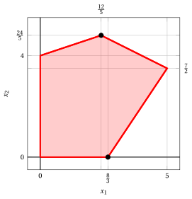
A feasible dual solution is:
It provides the following upper bound on the optimal value:
Another feasible dual solution is:
It provides the following upper bound on the optimal value:
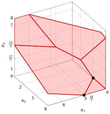
-
Using Weak Duality, we can show that \((\tilde x_1,\tilde x_2,\dots,\tilde x_n)\) is an optimal solution of the primal problem (9.1) and \((\tilde \pi_1,\tilde \pi_2,\dots,\tilde \pi_m)\) is an optimal solution of the dual problem (9.2) if they are feasible for their respective problems and satisfy
\[ \sum_{j=1}^n c_j \tilde x_j = \sum_{i=1}^m b_i \tilde \pi_i. \]This follows from Weak Duality as follows:
-
By Weak Duality, for every feasible solution \((\bar x_1,\bar x_2,\dots,\bar x_n)\) of the primal problem (9.1), and for the feasible dual solution \((\tilde \pi_1,\tilde \pi_2,\dots,\tilde \pi_m)\), we have
\[ \sum_{j=1}^n c_j \bar x_j \le \sum_{i=1}^m b_i \tilde \pi_i. \]If, in addition,
\[ \sum_{j=1}^n c_j \tilde x_j = \sum_{i=1}^m b_i \tilde \pi_i, \]then
\[ \sum_{j=1}^n c_j \bar x_j \le \sum_{j=1}^n c_j \tilde x_j \]for every feasible solution \((\bar x_1,\bar x_2,\dots,\bar x_n)\) of the primal problem. Hence, \((\tilde x_1,\tilde x_2,\dots,\tilde x_n)\) is an optimal solution of the primal problem (9.1).
-
By Weak Duality, for every feasible solution \((\bar \pi_1,\bar \pi_2,\dots,\bar \pi_m)\) of the dual problem (9.2), and for the feasible primal solution \((\tilde x_1,\tilde x_2,\dots,\tilde x_n)\), we have
\[ \sum_{j=1}^n c_j \tilde x_j \le \sum_{i=1}^m b_i \bar \pi_i. \]If, in addition,
\[ \sum_{j=1}^n c_j \tilde x_j = \sum_{i=1}^m b_i \tilde \pi_i, \]then
\[ \sum_{i=1}^m b_i \tilde \pi_i \le \sum_{i=1}^m b_i \bar \pi_i \]for every feasible solution \((\bar \pi_1,\bar \pi_2,\dots,\bar \pi_m)\) of the dual problem. Hence, \((\tilde \pi_1,\tilde \pi_2,\dots,\tilde \pi_m)\) is an optimal solution of the dual problem (9.2).
-
Example 9.5: Primal and dual optimal solutions
Consider the following pair of primal and dual LP problems:
To show that
is an optimal solution of the primal problem (9.1), and that
is an optimal solution of the dual problem (9.2), we can proceed as follows.
First, we verify that we have a feasible solution for the primal problem:
Second, we verify that we have a feasible solution for the dual problem:
Finally, we compute the objective function values:
and
Since both solutions are feasible for their respective problems and their objective values are equal, by Weak Duality, they are both optimal.
9.1.2 Strong Duality
- The following theorem, called Strong Duality, states that the primal problem (9.1) has an optimal solution if and only if the dual problem (9.2) has an optimal solution, and in this case, the optimal values of the two problems coincide.
Theorem 9.4: Strong Duality
The primal problem (9.1) has an optimal solution \((\tilde x_1,\tilde x_2,\dots,\tilde x_n)\) if and only if the dual problem (9.2) has an optimal solution \((\tilde \pi_1,\tilde \pi_2,\dots,\tilde \pi_m)\), and in this case
-
The existence of an optimal solution does not imply its uniqueness. This theorem only states that there exists at least one optimal solution for the primal problem if and only if there exists at least one optimal solution for the dual problem (there may be several optimal solutions on one side or on both sides, but the optimal objective values are equal).
-
Strong duality implies that
\[ \begin{array}{c} \text{the primal problem has an optimal solution}\\[1ex] \Updownarrow \\[1ex] \text{the dual problem has an optimal solution} \end{array} \]so “the primal problem has an optimal solution” is a necessary and sufficient condition to “the dual problem has an optimal solution” and vice versa.
-
The main steps of the proof of the Strong Duality theorem are as follows:
-
We first show that if the primal problem has an optimal solution, then the dual problem has an optimal solution, and the optimal values of the two problems coincide.
This is done by using an optimal dictionary of the primal problem produced by the simplex algorithm to construct a feasible solution of the dual problem satisfying \(\eqref{SD}\).
By Weak Duality, such a dual solution is necessarily optimal, which proves one implication.
-
The converse implication is obtained by applying the previous reasoning to the dual problem (equivalently, by exchanging the roles of primal and dual, since the dual of the dual is the primal problem).
-
Proof
Assume that the primal problem (9.1) has an optimal solution, and consider an optimal dictionary produced by the simplex algorithm. Its last row can be written as
Thus, \(\hat c_j\) is equal to the reduced cost of a variable \(x_j\) if \(j \in \pazocal{N}\) (the set of indices of the non-basic variables), and it is equal to \(0\) otherwise.
Rearranging the terms, we get
where the sum has been split into the original variables and the slack variables. Recall that, for the slack variables, we have
Substituting these expressions into the previous identity, we obtain
Since \(\eqref{A}\) is an identity in the variables \(x_1,x_2,\dots,x_n\), it holds for every choice of these variables. Therefore, the constant terms on the two sides must coincide, and the coefficients of each variable must also coincide. Hence,
and
Now we define
and we show that \((\tilde \pi_1,\tilde \pi_2,\dots,\tilde \pi_m)\) is an optimal solution of the dual problem (9.2) satisfying \(\eqref{SD}\).
Since the dictionary is optimal, we have \(\hat c_j \le 0\) for all \(j \in \{1,2,\dots,n+m\}\). Hence, from \(\eqref{D}\) we obtain
and from \(\eqref{C}\) we get
Therefore, \((\tilde \pi_1,\tilde \pi_2,\dots,\tilde \pi_m)\) is feasible for the dual problem (9.2).
Moreover, since \((\tilde x_1,\tilde x_2,\dots,\tilde x_n)\) is an optimal solution of the primal problem (9.1), its objective value is equal to the optimal value \(\bar z\) of the primal problem (9.1). Hence, by \(\eqref{B}\), we have
Thus, the feasible dual solution \((\tilde \pi_1,\tilde \pi_2,\dots,\tilde \pi_m)\) satisfies \(\eqref{SD}\).
Finally, Weak Duality implies that for every feasible dual solution \((\bar \pi_1,\bar \pi_2,\dots,\bar \pi_m)\),
Since for the feasible dual solution \((\tilde \pi_1,\tilde \pi_2,\dots,\tilde \pi_m)\) we have
it follows that
for every feasible dual solution \((\bar \pi_1,\bar \pi_2,\dots,\bar \pi_m)\). Hence, \((\tilde \pi_1,\tilde \pi_2,\dots,\tilde \pi_m)\) is an optimal solution of the dual problem (9.2).
The converse implication is obtained by applying the previous reasoning to the dual problem (after rewriting it in the corresponding canonical form, if needed). Since the dual of the dual problem is the primal problem, it follows that if the dual problem (9.2) has an optimal solution, then the primal problem (9.1) also has an optimal solution. □
-
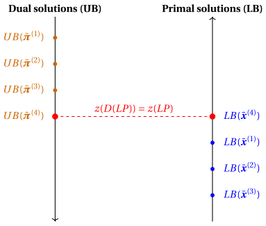
The figure below illustrates the relationship between primal and dual bounds for a maximization LP problem. As an illustrative example, the figure considers four primal feasible solutions
\[ \bar{\boldsymbol x}^{(1)}, \bar{\boldsymbol x}^{(2)}, \bar{\boldsymbol x}^{(3)}, \bar{\boldsymbol x}^{(4)}, \]and four dual feasible solutions
\[ \bar{\boldsymbol\pi}^{(1)}, \bar{\boldsymbol\pi}^{(2)}, \bar{\boldsymbol\pi}^{(3)}, \bar{\boldsymbol\pi}^{(4)}. \]Primal feasible solutions provide lower bounds on the optimal value, while dual feasible solutions provide upper bounds on the optimal value by the Weak Duality theorem \(\eqref{WD}\).
The fourth solution of each sequence attains the optimal value, and by the Strong Duality theorem \(\eqref{SD}\) the two bounds meet: \(z(\,{ LP}\,) = z(~{ D(LP)}~)\).
Example 9.6: optimal dual solutions from primal optimal dictionaries
Let us consider the primal problem of Example 9.1 (where \(n=2\) and \(m=3\)). The standard form of the primal problem is
where \(x_3\), \(x_4\) and \(x_5\) are the slack variables associated with the three constraints. An optimal dictionary reads as follows:
where the basic variables are \(x_1\), \(x_2\) and \(x_3\), and the non-basic variables are \(x_4\) and \(x_5\). The optimal primal solution is \(\tilde{x}_1=5\), \(\tilde{x}_2=\frac{7}{2}\), \(\tilde{x}_3=\frac{13}{2}\), \(\tilde{x}_4=0\) and \(\tilde{x}_5=0\), and the optimal value is \(32\).
The dual problem is
The values \(\hat{c}_j\) with \(j \in \{1,2,3,4,5\}\) used in the proof of the Strong Duality theorem are:
The optimal dual solution can be obtained by assigning the values \(\hat{c}_j\) to the corresponding dual variables with reversed signs, as in \(\eqref{D}\), and it reads as follows:
The solution is feasible for the dual problem, since \(\tilde{\pi}_1\), \(\tilde{\pi}_2\) and \(\tilde{\pi}_3\) are non-negative and
The objective function value of this solution is:
9.2 Primal and dual problems: possible outcomes
- The Weak Duality and the Strong Duality theorems relate the optimal values of the primal problem (9.1) and of the dual problem (9.2) whenever both admit an optimal solution. We now describe what happens when one of the two problems is infeasible or unbounded.
Corollary 9.5: unbounded problems and infeasible problems
For a pair of primal (9.1) and dual (9.2) problems:
-
if the primal problem is unbounded, then the dual problem is infeasible;
-
if the dual problem is unbounded, then the primal problem is infeasible.
- The idea of the proof is that one single feasible solution of one of the two problems would bound the objective value of the other one, by Weak Duality.
Proof
We prove the first point; the second one is obtained by exchanging the roles of the two problems.
Assume, by contradiction, that the primal problem (9.1) is unbounded and that the dual problem (9.2) admits a feasible solution \((\bar \pi_1,\bar \pi_2,\dots,\bar \pi_m)\). By Weak Duality \(\eqref{WD}\), for every feasible solution \((\bar x_1,\bar x_2,\dots,\bar x_n)\) of the primal problem we have
where \(M\) is a fixed real number, since the dual feasible solution is fixed. Accordingly, no feasible solution of the primal problem has an objective value larger than \(M\), which contradicts the assumption that the primal problem is unbounded. □
Theorem 9.6: possible outcomes of a pair of primal and dual problems
For a pair of primal (9.1) and dual (9.2) problems, exactly one of the following four cases occurs:
-
both problems admit an optimal solution, and the two optimal values coincide;
-
the primal problem is unbounded and the dual problem is infeasible;
-
the primal problem is infeasible and the dual problem is unbounded;
-
both problems are infeasible.
Proof
By the Fundamental Theorem of Linear Programming, each of the two problems is infeasible, is unbounded, or admits an optimal solution, and then there are nine possible combinations. We show that five of them cannot occur.
-
If the primal problem admits an optimal solution, then by Strong Duality \(\eqref{SD}\) the dual problem admits an optimal solution as well. This excludes the two combinations in which the primal problem admits an optimal solution and the dual problem is unbounded or infeasible. Symmetrically, the two combinations in which the dual problem admits an optimal solution and the primal problem is unbounded or infeasible are excluded as well.
-
If the primal problem is unbounded, then by Corollary 9.5 the dual problem is infeasible. This excludes the combination in which both problems are unbounded.
The four remaining combinations are the ones of the statement. □
The possible outcomes of a pair of primal and dual problems are summarized in the following table, where the four cases of Theorem 9.6 are marked by ✓:
| dual problem \(D(LP)\) | |||
|---|---|---|---|
| primal problem \(LP\) | optimal solution | unbounded | infeasible |
| optimal solution | ✓ | ||
| unbounded | ✓ | ||
| infeasible | ✓ | ✓ | |
In particular, an infeasible primal problem may have either an unbounded or an infeasible dual problem: the infeasibility of the primal problem alone does not determine the outcome of the dual problem.
Example 9.7: unbounded primal problem and infeasible dual problem
Consider the following pair of primal and dual problems, with \(n=2\) and \(m=2\) (called Example 9.7):
The primal problem is unbounded: for every value \(t \ge 0\), the point \(\bar x_1 = \bar x_2 = t\) is a feasible solution of objective value \(2 \, t\).
The dual problem is infeasible: by summing its two constraints we obtain
which is never satisfied.
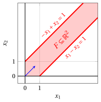
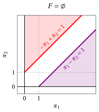
In the first figure the feasible region of the primal problem, in the second one the two half-planes defined by the dual constraints, whose intersection is empty.
Example 9.8: infeasible primal problem and unbounded dual problem
Consider the following pair of primal and dual problems, with \(n=2\) and \(m=2\) (called Example 9.8):
The primal problem is infeasible: the first constraint imposes \(x_1 + x_2 \le 2\) and the second one imposes \(x_1 + x_2 \ge 4\).
The dual problem is unbounded: for every value \(t \ge 0\), the point \(\bar \pi_1 = 1 + t\) and \(\bar \pi_2 = t\) is a feasible solution, since \(\bar \pi_1 - \bar \pi_2 = 1 \ge 1\), and its objective value is
which tends to \(-\infty\) as \(t\) grows. Since the dual problem is a minimization problem, it is unbounded.
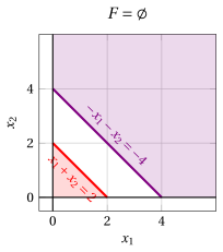
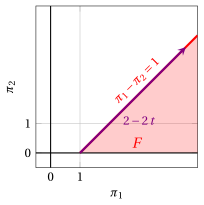
In the first figure the two half-planes defined by the primal constraints, whose intersection is empty; in the second one the feasible region of the dual problem and, in violet, the family of feasible solutions along which its objective value tends to \(-\infty\).
Example 9.9: infeasible primal problem and infeasible dual problem
Consider the following pair of primal and dual problems, with \(n=2\) and \(m=2\) (called Example 9.9):
The primal problem is infeasible: the two constraints impose \(x_1 - x_2 \le 1\) and \(x_1 - x_2 \ge 2\).
The dual problem is infeasible as well: by summing its two constraints we obtain \(0 \ge 2\), which is never satisfied.
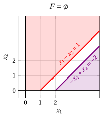
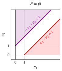
In the first figure the primal problem and in the second one the dual problem: both feasible regions are empty.
Theorem 9.6 can be used to certify the outcome of an LP problem:
-
one feasible solution of the dual problem proves that the primal problem is not unbounded;
-
one feasible solution of the primal problem proves that the dual problem is not unbounded;
-
one feasible solution of each of the two problems proves that both admit an optimal solution.
9.3 Complementary Slackness
- The following theorem, called Complementary Slackness, states that a feasible solution of the primal problem (9.1) and a feasible solution of the dual problem (9.2) are both optimal if and only if the Complementary Slackness Conditions hold.
Theorem 9.7: Complementary Slackness
A feasible solution \((\bar x_1,\bar x_2,\dots,\bar x_n)\) of the primal problem (9.1) and a feasible solution \((\bar \pi_1,\bar \pi_2,\dots,\bar \pi_m)\) of the dual problem (9.2) are optimal solutions of their respective problems if and only if the following conditions hold:
- In \(\eqref{WW}\) and \(\eqref{QQ}\), the “or” is inclusive, that is, both conditions may hold simultaneously.
Definition 9.8: Complementary Slackness Conditions
Conditions \(\eqref{WW}\) and \(\eqref{QQ}\) are called Complementary Slackness Conditions and they can be equivalently rewritten as:
-
Complementary Slackness implies that
\[ \begin{array}{c} \text{a pair of primal and dual feasible solutions are optimal}\\[1ex] \Updownarrow \\[1ex] \text{the Complementary Slackness Conditions hold} \end{array} \]so “the Complementary Slackness Conditions hold” is a necessary and sufficient condition for “a pair of feasible primal and dual solutions are optimal” and vice versa.
Definition 9.9: active constraints
A primal or a dual constraint is called:
-
active if it is satisfied at equality by a given solution (there is no slack);
-
not active if it is not satisfied at equality by a given solution (there is a slack).
-
Condition \(\eqref{WW}\) (or equivalently \(\eqref{WW_bis}\)) implies that if a primal constraint is not active, i.e., there is a slack, the corresponding dual variable must be zero.
-
Condition \(\eqref{QQ}\) (or equivalently \(\eqref{QQ_bis}\)) implies that if a dual constraint is not active, i.e., there is a slack, the corresponding primal variable must be zero.
Example 9.10: Complementary slackness
Consider the following pair of primal and dual LP problems:
An optimal primal solution is
Primal slacks:
The first primal constraint is not active, i.e., there is a slack. So the corresponding dual variable \(\tilde\pi_1\) must be zero.
The second and third primal constraints are active, i.e., there are no slacks. So the corresponding dual variables \(\tilde\pi_2\) and \(\tilde\pi_3\) are free to be positive.
An optimal dual solution is
Dual slacks:
All dual constraints are active, i.e., there are no slacks. So the corresponding primal variables \(\tilde x_1\) and \(\tilde x_2\) are free to be positive.
-
The complementary slackness conditions geometrically mean that, given an optimal solution (\(\tilde x_1,\tilde x_2,\dots,\tilde x_n\)) of a primal problem (9.1) and an optimal solution (\(\tilde \pi_1,\tilde \pi_2,\dots,\tilde \pi_m\)) of its dual problem (9.2), we have two pairs of perpendicular vectors:
\[ \begin{pmatrix} \tilde{\pi}_1 \\ \tilde{\pi}_2 \\ \vdots \\ \tilde{\pi}_m \end{pmatrix}, ~~~~~~ \begin{pmatrix} \displaystyle \sum_{j=1}^n a_{1j} \tilde x_j - b_1 \\ \displaystyle \sum_{j=1}^n a_{2j} \tilde x_j - b_2 \\ \vdots \\ \displaystyle \sum_{j=1}^n a_{mj} \tilde x_j - b_m \end{pmatrix} \text{ and } \begin{pmatrix} \tilde{x}_1 \\ \tilde{x}_2 \\ \vdots \\ \tilde{x}_n \end{pmatrix}, ~~~~~ \begin{pmatrix} c_1 - \displaystyle \sum_{i=1}^m a_{i1} \tilde \pi_i \\ c_2 - \displaystyle \sum_{i=1}^m a_{i2} \tilde \pi_i \\ \vdots \\ c_n - \displaystyle \sum_{i=1}^m a_{in} \tilde \pi_i \end{pmatrix} \]
Example 9.11: Complementary Slackness
Consider again the previous pair of primal and dual LP problems and their optimal solutions.
The first pair of perpendicular vectors (nonzero case) is
Orthogonality check:
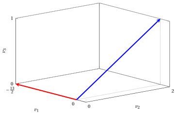
The two vectors are drawn in the same space \(\R^3\) with generic coordinates \((v_1, v_2, v_3)\): in blue the optimal dual solution \(\tilde{\boldsymbol \pi}\), in red the vector of the primal constraint values minus the RHS, \(\left(-\frac{13}{2}, 0, 0\right)\).
The second pair of perpendicular vectors is
Orthogonality check:
Proof
Since \((\bar x_1,\bar x_2,\dots,\bar x_n)\) is a feasible solution of the primal problem (9.1) and \((\bar \pi_1,\bar \pi_2,\dots,\bar \pi_m)\) is a feasible solution of the dual problem (9.2), by the same argument used in the proof of Weak Duality, we have
The first inequality of \(\eqref{KKK}\) can be rewritten as
and by dual feasibility and primal feasibility, for all \(j \in \{1,2,\dots,n\}\), we have
A sum of non-negative terms equals zero if and only if each term is zero. Therefore, equality holds in the first inequality of \(\eqref{KKK}\) if and only if
that is, if and only if condition \(\eqref{QQ}\) holds.
Similarly, the second inequality of \(\eqref{KKK}\) can be rewritten as
and by primal feasibility and dual feasibility, for all \(i \in \{1,2,\dots,m\}\), we have
A sum of non-negative terms equals zero if and only if each term is zero. Therefore, equality holds in the second inequality of \(\eqref{KKK}\) if and only if
that is, if and only if condition \(\eqref{WW}\) holds.
Assume first that \((\bar x_1,\bar x_2,\dots,\bar x_n)\) and \((\bar \pi_1,\bar \pi_2,\dots,\bar \pi_m)\) are optimal solutions of their respective problems. Then, by Strong Duality,
Therefore, both inequalities in \(\eqref{KKK}\) must hold with equality, and hence conditions \(\eqref{WW}\) and \(\eqref{QQ}\) hold.
Conversely, assume that conditions \(\eqref{WW}\) and \(\eqref{QQ}\) hold. Then both inequalities in \(\eqref{KKK}\) hold with equality, and therefore
Since \((\bar x_1,\bar x_2,\dots,\bar x_n)\) and \((\bar \pi_1,\bar \pi_2,\dots,\bar \pi_m)\) are feasible solutions, Weak Duality implies that they are optimal solutions of their respective problems. □
- The following theorem (derived from the previous one) allows us to check whether a feasible solution of a primal problem (9.1) is optimal by constructing (if possible) a feasible solution of the dual problem (9.2) with the same objective function value, i.e., it is an optimality check.
Corollary 9.10
A feasible solution \((\bar x_1,\bar x_2,\dots,\bar x_n)\) of the primal problem (9.1) is optimal if and only if there exists \((\bar \pi_1,\bar \pi_2,\dots,\bar \pi_m)\) such that:
Proof
Assume first that \((\bar x_1,\bar x_2,\dots,\bar x_n)\) is an optimal solution of problem (9.1).
By Strong Duality, there exists an optimal solution \((\bar \pi_1,\bar \pi_2,\dots,\bar \pi_m)\) of the dual problem (9.2). Since \((\bar \pi_1,\bar \pi_2,\dots,\bar \pi_m)\) is feasible for the dual problem, it satisfies \(\eqref{ZZ3}\) and \(\eqref{ZZ4}\).Moreover, since the primal and dual solutions are both optimal, by Complementary Slackness they satisfy \(\eqref{ZZ1}\) and \(\eqref{ZZ2}\).
Hence, there exists \((\bar \pi_1,\bar \pi_2,\dots,\bar \pi_m)\) satisfying \(\eqref{ZZ1}\)–\(\eqref{ZZ4}\).
Conversely, assume that there exists \((\bar \pi_1,\bar \pi_2,\dots,\bar \pi_m)\) satisfying \(\eqref{ZZ1}\)–\(\eqref{ZZ4}\).
Since \((\bar x_1,\bar x_2,\dots,\bar x_n)\) is feasible for the primal problem by hypothesis, and \(\eqref{ZZ3}\)–\(\eqref{ZZ4}\) imply that \((\bar \pi_1,\bar \pi_2,\dots,\bar \pi_m)\) is feasible for the dual problem, both vectors are feasible for their respective problems. Furthermore, \(\eqref{ZZ1}\) implies condition \(\eqref{QQ}\). Moreover, primal feasibility together with \(\eqref{ZZ2}\) implies condition \(\eqref{WW}\).
Therefore, the primal and dual feasible solutions satisfy the Complementary Slackness conditions, and by the Complementary Slackness theorem they are optimal for their respective problems. □
Example 9.12: Complementary Slackness
We check if the feasible solution
of the LP problem of Example 9.1 is optimal.
-
Since
\[ \sum_{i=1}^m a_{ij} \bar \pi_i = c_j \text{ if }\bar x_j>0,~\forall j \in \{1,2,\dots,n\} \]we build the following system of two linear equations with three variables:
\[ \begin{array}{rrrrrrrrrrrrr} & {-} \, {\bar \pi_1} & {+} & \, {\bar \pi_2} & {+} & 3 \, {\bar \pi_3} & {=} & 5 & & {\left(\bar x_1=5>0\right)} \\[2ex] & 3\, {\bar \pi_1} & {+} & 2 \, {\bar \pi_2} & {-} & 2 \, {\bar \pi_3} & {=} & 2 & & {\left(\bar x_2=\frac{7}{2}>0\right)} \end{array} \] -
Since
\[ \bar \pi_i = 0 \text{ if } \sum_{j=1}^n a_{ij} \bar x_j < b_i,~\forall i \in \{1,2,\dots,m\} \]we compute:
\[ \begin{array}{rrrrrrrrrrrrr} & {-1} {\cdot} {5} & {+} & 3 {\cdot} {\frac{7}{2}} & {=} & {\frac{11}{2}< 12} & { \text{ so } \bar \pi_1 = 0} \\[2ex] & 1 {\cdot} {5} & {+} & 2 {\cdot} {\frac{7}{2}} & {=} & {12 \nless 12} & \\[2ex] & 3 {\cdot} {5} & {-} & 2 {\cdot} {\frac{7}{2}} & {=} & {8 \nless 8} & \end{array} \]We then solve the previous system of two equations with two variables and we get:
\[ \bar{\pi}_1=0,~~ \bar{\pi}_2=2,~~\bar{\pi}_3=1 \] -
We need to check
\[ \sum_{i=1}^m a_{ij} \bar \pi_i \ge c_j, \quad \forall j \in \{1,2,\dots,n\} \]so we compute:
\[ \begin{array}{rrrrrrrrrrrrr} & {-1} {\cdot} {0} & {+} & 1 {\cdot} {2} & {+} & 3 {\cdot} {1} & {=} & 5 { \ge 5} \\[2ex] & {3} {\cdot} {0} & {+} & 2 {\cdot} {2} & {-} & 2 {\cdot} {1} & {=} & 2 { \ge 2} \end{array} \] -
We need to check
\[ \bar \pi_i \ge 0, \quad \forall i \in \{1,2,\dots,m\} \]so since
\[ \bar \pi_1=0 \ge 0, ~~\bar \pi_2=2 \ge 0, ~~\bar \pi_3=1 \ge 0 \]the solution is optimal.
Example 9.13: Complementary Slackness
We check if the feasible solution
of the LP problem of Example 9.1 is optimal.
-
Since
\[ \sum_{i=1}^m a_{ij} \bar \pi_i = c_j \text{ if }\bar x_j>0,~\forall j \in \{1,2,\dots,n\} \]we build the following system of two linear equations with three variables:
\[ \begin{array}{rrrrrrrrrrrrr} & {-} \, {\bar \pi_1} & {+} & \, {\bar \pi_2} & {+} & 3 \, {\bar \pi_3} & {=} & 5 & & {\left(\bar x_1=\frac{12}{5}>0\right)} \\[2ex] & 3\, {\bar \pi_1} & {+} & 2 \, {\bar \pi_2} & {-} & 2 \, {\bar \pi_3} & {=} & 2 & & {\left(\bar x_2=\frac{24}{5}>0\right)} \end{array} \] -
Since
\[ \bar \pi_i = 0 \text{ if } \sum_{j=1}^n a_{ij} \bar x_j < b_i,~\forall i \in \{1,2,\dots,m\} \]we compute:
\[ \begin{array}{rrrrrrrrrrrrr} & {-1} {\cdot} {\frac{12}{5}} & {+} & 3 {\cdot} {\frac{24}{5}} & {=} & {12 \nless 12} & \\[2ex] & 1 {\cdot} {\frac{12}{5}} & {+} & 2 {\cdot} {\frac{24}{5}} & {=} & {12 \nless 12} & \\[2ex] & 3 {\cdot} {\frac{12}{5}} & {-} & 2 {\cdot} {\frac{24}{5}} & {=} & {-\frac{12}{5}< 8} & { \text{ so } \bar \pi_3 = 0} \end{array} \]We then solve the previous system of two equations with two variables and we get:
\[ \bar{\pi}_1 = -\frac{8}{5},~~\bar{\pi}_2 = \frac{17}{5},~~\bar{\pi}_3=0 \] -
We need to check
\[ \sum_{i=1}^m a_{ij} \bar \pi_i \ge c_j, \quad \forall j \in \{1,2,\dots,n\} \]so we compute:
\[ \begin{array}{rrrrrrrrrrrrr} & {-1} {\cdot} {\left(-\frac{8}{5}\right)} & {+} & 1 {\cdot} {\frac{17}{5}} & {+} & 3 {\cdot} {0} & {=} & 5 { \ge 5} \\[2ex] & {3} {\cdot} {\left(-\frac{8}{5}\right)} & {+} & 2 {\cdot} {\frac{17}{5}} & {-} & 2 {\cdot} {0} & {=} & 2 { \ge 2} \end{array} \] -
We need to check
\[ \bar \pi_i \ge 0, \quad \forall i \in \{1,2,\dots,m\} \]but since
\[ \bar \pi_1=-\frac{8}{5} < 0 \]the solution is not optimal.
9.3.1 Dual problem in matrix notation
-
The input data of an LP problem in canonical maximization form with \(n\) variables and \(m\) less-than-or-equal-to inequality constraints can be represented in matrix notation by an objective-function coefficient vector \({\boldsymbol c} \in \R^n\) of \(n\) rows, by an RHS vector \({\boldsymbol b} \in \R^m\) of \(m\) rows, and by a constraint matrix \({\boldsymbol A} \in \R^{m \times n}\) with \(m\) rows and \(n\) columns:
\[ {\boldsymbol c}= \begin{pmatrix} c_{1} \\ c_{2} \\ \vdots \\ \vdots \\ c_{n} \\ \end{pmatrix} \qquad\qquad {\boldsymbol A}= \begin{pmatrix} a_{11} & a_{12} & \dots& \dots & a_{1n}\\ a_{21} & a_{22} & \dots& \dots & a_{2n}\\ \vdots & \vdots & \dots& \dots & \vdots \\ a_{m1} & a_{m2} & \dots& \dots & a_{mn}\\ \end{pmatrix} \qquad\qquad {\boldsymbol b}= \begin{pmatrix} b_{1} \\ b_{2} \\ \vdots \\ b_{m} \\ \end{pmatrix} \] -
The \(n\) primal variables can be represented by a column vector \({\boldsymbol x} \in \R^n\) of \(n\) rows containing the \(n\) variables, and the \(m\) dual variables can be represented by a column vector \(\boldsymbol{\pi} \in \R^m\) of \(m\) rows containing the \(m\) variables:
\[ {\boldsymbol x}= \begin{pmatrix} x_{1} \\ x_{2} \\ \vdots \\ \vdots \\ x_{n} \\ \end{pmatrix} \qquad\qquad \boldsymbol{\pi} = \begin{pmatrix} \pi_{1} \\ \pi_{2} \\ \vdots \\ \pi_{m} \\ \end{pmatrix} \] -
Using matrix notation, a primal problem in canonical maximization form and its dual problem read as follows:
\[\begin{align*} && \max \;\;{\boldsymbol c}'\; {\boldsymbol x} \\[2ex] && \text{subject to} \quad {\boldsymbol A} \; {\boldsymbol x} &\leq {\boldsymbol b}, \\[2ex] && {\boldsymbol x} &\ge {\boldsymbol 0}. \end{align*}\]\[\begin{align*} && \min \;\;{\boldsymbol b}' \; \boldsymbol{\pi} \\[2ex] && \text{subject to} \quad {\boldsymbol A}' \; \boldsymbol{\pi} &\geq {\boldsymbol c}, \\[2ex] && \boldsymbol{\pi} &\ge {\boldsymbol 0}. \end{align*}\]
Example 9.14: matrix notation
For the LP problem of Example 9.1, with \(n=2\) variables and \(m=3\) constraints, the input data are:
and the variables are:
9.4 Dual problem of a generic LP problem
Definition 9.11: dual problem of a generic LP problem
Given the following generic LP problem:
where
-
\(N_{\ge 0}\), \(N_{\gtreqless 0}\) and \(N_{\le 0}\) are the disjoint subsets of indices of the non-negative, free and nonpositive variables, respectively, and \(N= N_{\ge 0} \cup N_{\gtreqless 0} \cup N_{\le 0}\);
-
\(M_{\le}\), \(M_{=}\) and \(M_{\ge}\) are the disjoint subsets of indices of the less-than-or-equal-to, equality and greater-than-or-equal-to constraints, respectively, and \(M= M_{\le } \cup M_{=} \cup M_{\ge}\).
the dual problem \(D(LP)\) of the LP problem (9.8) is the following LP problem:
Example 9.15: dual problem of a generic LP problem
Consider the following generic LP problem:
As far as the index of the variables is concerned, we have:
As far as the index of the constraints is concerned, we have:
The dual problem \(D(LP)\) of the LP problem is:
Since an equivalent LP problem in canonical maximization form can be obtained from an LP in generic maximization form, Weak Duality, Strong Duality, and the Complementary Slackness theorem hold for the generic case as well.
Exercises on this chapter: Duality theory
Interactive lab
The ideas of the chapter, hands on: move the sliders and drag the points. Each app also opens full page in the interactive lab: Weak and strong duality.