Exercises · Revised simplex algorithm

Exercises · Chapter 11 · each solution opens with a click · Chapter 11: Revised simplex algorithm · Exercises, volume 4 (PDF)

Problems with two variables

Exercise 11.1: Revised simplex algorithm (P0)

Consider the following LP problem in canonical maximization form with \(n=2\) variables and \(m=1\) constraint:

\[ \begin{array}{rrrrrr} {\max} & {2}\, {x_1} & {+} & {4}\, {x_2} \\[2ex] \text{subject to} & {2}\, {x_1} & {+} & {3}\, {x_2} & {\le} & {4} \\[2ex] & {x_1,} & & {x_2} & {\ge} & {0} \end{array} \]

By introducing the slack variable, we get the following LP problem in standard maximization form with \(n+m=3\) variables and \(m=1\) constraint:

\[ \begin{array}{rrrrrrrr} {\max} & {2}\, {x_1} & {+} & {4}\, {x_2} \\[2ex] \text{subject to} & {2}\, {x_1} & {+} & {3}\, {x_2} & {+} & {x_3} & {=} & {4} \\[2ex] & {x_1,} & & {x_2,} & & {x_3} & {\ge} & {0} \end{array} \]

Questions

• Execute the revised simplex algorithm to find an optimal solution of this LP problem using Bland's rule to select the pivot column and the pivot row.

Solution

We have:

\[ {\boldsymbol A}= \begin{pmatrix} 2 & 3 & 1 \end{pmatrix} \quad {\boldsymbol b}= \begin{pmatrix} 4 \end{pmatrix} \quad {\boldsymbol c}= \begin{pmatrix} 2\\ 4\\ 0 \end{pmatrix} \quad {\boldsymbol x}= \begin{pmatrix} x_1 \\ x_2 \\ x_3 \end{pmatrix} \]

• Initialization

  Since it is an LP problem in standard form obtained from an LP problem in canonical form with \(~{\boldsymbol b} \ge 0\) by adding the slack variables, the partition \(\pazocal{B}=\{3\}\) and \(\pazocal{N}=\{1,2\}\) is associated with the following basic feasible solution:

  \[ \begin{pmatrix} x_3 \end{pmatrix} = \begin{pmatrix} 4 \end{pmatrix} \text{ and } \begin{pmatrix} x_1 \\ x_2 \end{pmatrix} = \begin{pmatrix} 0\\ 0 \end{pmatrix} \]

• Iteration 1

  With \(\pazocal{B}= \{3\}\) and \(\pazocal{N}= \{1,~~2\}\), we have:

  \[ {\boldsymbol x}_{\pazocal{B}}= \begin{pmatrix} x_3 \end{pmatrix} ~~ {\boldsymbol A}_{\pazocal{B}}= \begin{pmatrix} 1 \end{pmatrix} ~~ {\boldsymbol c}_{\pazocal{B}}= \begin{pmatrix} 0 \end{pmatrix} ~~ {{ \bar{\boldsymbol b}}}= \begin{pmatrix} 4 \end{pmatrix} \]
  \[ {\boldsymbol x}_{\pazocal{N}}= \begin{pmatrix} x_1 \\ x_2 \end{pmatrix} ~~ {\boldsymbol A}_{\pazocal{N}}= \begin{pmatrix} 2 & 3 \end{pmatrix} ~~ {\boldsymbol c}_{\pazocal{N}}= \begin{pmatrix} 2\\ 4 \end{pmatrix} \]

  Optimality check

  We solve \({\boldsymbol \pi} \; {\boldsymbol A}_{\pazocal{B}} = {\boldsymbol c}'_{\pazocal{B}}\) to compute \({\boldsymbol \pi} = {{{\boldsymbol c}'_{\pazocal{B}} \; {\boldsymbol A}_{\pazocal{B}}^{-1}}}\), first system of linear equations:

  \[\begin{equation*} \begin{cases} \begin{array}{rrr} {\pi_3} & {=} & {0} \end{array} \end{cases} \qquad {\boldsymbol \pi}= \begin{pmatrix} 0\\ \end{pmatrix} \end{equation*}\]

  We compute the basic feasible solution value \({\bar{z}} = {\boldsymbol \pi} \; {\boldsymbol b} = \begin{pmatrix} 0\\ \end{pmatrix} \begin{pmatrix} 4 \end{pmatrix} = 0\)

  We compute the reduced costs \({{ \bar{\boldsymbol c}}'} = {{\boldsymbol c}'_{\pazocal{N}} - {\boldsymbol \pi} \; {\boldsymbol A}_{\pazocal{N}}}\):

  \[ {{ \bar{\boldsymbol c}}'} = \begin{pmatrix} 2 & 4\\ \end{pmatrix} - \begin{pmatrix} 0\\ \end{pmatrix} \begin{pmatrix} 2 & 3 \end{pmatrix} = \underbrace{ \begin{pmatrix} 2 & 4\\ \end{pmatrix} }_{{c_{1}~~~c_{2}}} - \underbrace{ \begin{pmatrix} 0 & 0\\ \end{pmatrix} }_{{\boldsymbol \pi}\;{\boldsymbol A}_{1} ~~{\boldsymbol \pi}\;{\boldsymbol A}_{2}} = \underbrace{ \begin{pmatrix} 2 & 4\\ \end{pmatrix} }_{{\bar{c}_{1}~~~\bar{c}_{2}}} \]

  Not all reduced costs are non-positive then we perform a pivoting operation.

  Pivoting operation

  Since \({c}_{1} > {\boldsymbol \pi} \;{\boldsymbol A}_{1}\), \(x_1\) is the pivot column and we have \({\boldsymbol A}_{1} = \begin{pmatrix} 2 \end{pmatrix}\)

  We solve \({\boldsymbol A}_{\pazocal{B}} \; {\boldsymbol d} = {\boldsymbol A}_{1}\) to compute \({\boldsymbol d}={ {\boldsymbol A}_{\pazocal{B}}^{-1}} {\boldsymbol A}_{1}\), second system of linear equations:

  \[\begin{equation*} \begin{cases} \begin{array}{rrr} {d_3} & {=} & {2} \end{array} \end{cases} \qquad {\boldsymbol d}= \begin{pmatrix} 2 \end{pmatrix} \end{equation*}\]

  We have to find the largest \(t\) such that \({{ \bar{\boldsymbol b}}} - t \; {{\boldsymbol d}} \ge 0\):

  \[ \begin{cases} \underbrace{4 -t \cdot 2\ge 0}_{x_3 \ge 0} \end{cases} \qquad \begin{cases} t\le 2 \end{cases} \text{ then } t_{m}=2 \]

  Accordingly the value of the pivot column becomes \(t_{m}\), i.e., \(x_1=2\). The value of \(x_3\) becomes zero and \(x_3\) is the pivot row.

• Iteration 2

  With \(\pazocal{B}= \{1\}\) and \(\pazocal{N}= \{2,~~3\}\), we have:

  \[ {\boldsymbol x}_{\pazocal{B}}= \begin{pmatrix} x_1 \end{pmatrix} ~~ {\boldsymbol A}_{\pazocal{B}}= \begin{pmatrix} 2 \end{pmatrix} ~~ {\boldsymbol c}_{\pazocal{B}}= \begin{pmatrix} 2 \end{pmatrix} ~~ {{ \bar{\boldsymbol b}}}= \begin{pmatrix} 2 \end{pmatrix} \]
  \[ {\boldsymbol x}_{\pazocal{N}}= \begin{pmatrix} x_2 \\ x_3 \end{pmatrix} ~~ {\boldsymbol A}_{\pazocal{N}}= \begin{pmatrix} 3 & 1 \end{pmatrix} ~~ {\boldsymbol c}_{\pazocal{N}}= \begin{pmatrix} 4\\ 0 \end{pmatrix} \]

  Optimality check

  We solve \({\boldsymbol \pi} \; {\boldsymbol A}_{\pazocal{B}} = {\boldsymbol c}'_{\pazocal{B}}\) to compute \({\boldsymbol \pi} = {{{\boldsymbol c}'_{\pazocal{B}} \; {\boldsymbol A}_{\pazocal{B}}^{-1}}}\), first system of linear equations:

  \[\begin{equation*} \begin{cases} \begin{array}{rrr} {2}\, {\pi_1} & {=} & {2} \end{array} \end{cases} \qquad {\boldsymbol \pi}= \begin{pmatrix} 1\\ \end{pmatrix} \end{equation*}\]

  We compute the basic feasible solution value \({\bar{z}} = {\boldsymbol \pi} \; {\boldsymbol b} = \begin{pmatrix} 1\\ \end{pmatrix} \begin{pmatrix} 4 \end{pmatrix} = 4\)

  We compute the reduced costs \({{ \bar{\boldsymbol c}}'} = {{\boldsymbol c}'_{\pazocal{N}} - {\boldsymbol \pi} \; {\boldsymbol A}_{\pazocal{N}}}\):

  \[ {{ \bar{\boldsymbol c}}'} = \begin{pmatrix} 4 & 0\\ \end{pmatrix} - \begin{pmatrix} 1\\ \end{pmatrix} \begin{pmatrix} 3 & 1 \end{pmatrix} = \underbrace{ \begin{pmatrix} 4 & 0\\ \end{pmatrix} }_{{c_{2}~~~c_{3}}} - \underbrace{ \begin{pmatrix} 3 & 1\\ \end{pmatrix} }_{{\boldsymbol \pi}\;{\boldsymbol A}_{2} ~~{\boldsymbol \pi}\;{\boldsymbol A}_{3}} = \underbrace{ \begin{pmatrix} 1 & -1\\ \end{pmatrix} }_{{\bar{c}_{2}~~~\bar{c}_{3}}} \]

  Not all reduced costs are non-positive then we perform a pivoting operation.

  Pivoting operation

  Since \({c}_{2} > {\boldsymbol \pi} \;{\boldsymbol A}_{2}\), \(x_2\) is the pivot column and we have \({\boldsymbol A}_{2} = \begin{pmatrix} 3 \end{pmatrix}\)

  We solve \({\boldsymbol A}_{\pazocal{B}} \; {\boldsymbol d} = {\boldsymbol A}_{2}\) to compute \({\boldsymbol d}={ {\boldsymbol A}_{\pazocal{B}}^{-1}} {\boldsymbol A}_{2}\), second system of linear equations:

  \[\begin{equation*} \begin{cases} \begin{array}{rrr} {2}\, {d_1} & {=} & {3} \end{array} \end{cases} \qquad {\boldsymbol d}= \begin{pmatrix} \dfrac{3}{2} \end{pmatrix} \end{equation*}\]

  We have to find the largest \(t\) such that \({{ \bar{\boldsymbol b}}} - t \; {{\boldsymbol d}} \ge 0\):

  \[ \begin{cases} \underbrace{2 -t \cdot \dfrac{3}{2}\ge 0}_{x_1 \ge 0} \end{cases} \qquad \begin{cases} t\le \dfrac{4}{3} \end{cases} \text{ then } t_{m}=\dfrac{4}{3} \]

  Accordingly the value of the pivot column becomes \(t_{m}\), i.e., \(x_2=\dfrac{4}{3}\). The value of \(x_1\) becomes zero and \(x_1\) is the pivot row.

• Iteration 3

  With \(\pazocal{B}= \{2\}\) and \(\pazocal{N}= \{1,~~3\}\), we have:

  \[ {\boldsymbol x}_{\pazocal{B}}= \begin{pmatrix} x_2 \end{pmatrix} ~~ {\boldsymbol A}_{\pazocal{B}}= \begin{pmatrix} 3 \end{pmatrix} ~~ {\boldsymbol c}_{\pazocal{B}}= \begin{pmatrix} 4 \end{pmatrix} ~~ {{ \bar{\boldsymbol b}}}= \begin{pmatrix} \dfrac{4}{3} \end{pmatrix} \]
  \[ {\boldsymbol x}_{\pazocal{N}}= \begin{pmatrix} x_1 \\ x_3 \end{pmatrix} ~~ {\boldsymbol A}_{\pazocal{N}}= \begin{pmatrix} 2 & 1 \end{pmatrix} ~~ {\boldsymbol c}_{\pazocal{N}}= \begin{pmatrix} 2\\ 0 \end{pmatrix} \]

  Optimality check

  We solve \({\boldsymbol \pi} \; {\boldsymbol A}_{\pazocal{B}} = {\boldsymbol c}'_{\pazocal{B}}\) to compute \({\boldsymbol \pi} = {{{\boldsymbol c}'_{\pazocal{B}} \; {\boldsymbol A}_{\pazocal{B}}^{-1}}}\), first system of linear equations:

  \[\begin{equation*} \begin{cases} \begin{array}{rrr} {3}\, {\pi_2} & {=} & {4} \end{array} \end{cases} \qquad {\boldsymbol \pi}= \begin{pmatrix} \dfrac{4}{3}\\ \end{pmatrix} \end{equation*}\]

  We compute the basic feasible solution value \({\bar{z}} = {\boldsymbol \pi} \; {\boldsymbol b} = \begin{pmatrix} \dfrac{4}{3}\\ \end{pmatrix} \begin{pmatrix} 4 \end{pmatrix} = \dfrac{16}{3}\)

  We compute the reduced costs \({{ \bar{\boldsymbol c}}'} = {{\boldsymbol c}'_{\pazocal{N}} - {\boldsymbol \pi} \; {\boldsymbol A}_{\pazocal{N}}}\):

  \[ {{ \bar{\boldsymbol c}}'} = \begin{pmatrix} 2 & 0\\ \end{pmatrix} - \begin{pmatrix} \dfrac{4}{3}\\ \end{pmatrix} \begin{pmatrix} 2 & 1 \end{pmatrix} = \underbrace{ \begin{pmatrix} 2 & 0\\ \end{pmatrix} }_{{c_{1}~~~c_{3}}} - \underbrace{ \begin{pmatrix} \dfrac{8}{3} & \dfrac{4}{3}\\ \end{pmatrix} }_{{\boldsymbol \pi}\;{\boldsymbol A}_{1} ~~{\boldsymbol \pi}\;{\boldsymbol A}_{3}} = \underbrace{ \begin{pmatrix} -\dfrac{2}{3} & -\dfrac{4}{3}\\ \end{pmatrix} }_{{\bar{c}_{1}~~~\bar{c}_{3}}} \]

  All reduced costs are non-positive, then the basic feasible solution

  \[ {\boldsymbol x}_{\pazocal{B}}= \begin{pmatrix} x_2 \end{pmatrix}=\begin{pmatrix} \dfrac{4}{3} \end{pmatrix} \text{ and } {\boldsymbol x}_{\pazocal{N}}= \begin{pmatrix} x_1 \\ x_3 \end{pmatrix}=\begin{pmatrix} 0\\ 0 \end{pmatrix} \]

  is an optimal solution of the LP problem and \({\bar{z}} = \dfrac{16}{3}\) is the optimal solution value.

Graphical solution:

The feasible region of the LP problem (in canonical form) is the polyhedron shaded in red:

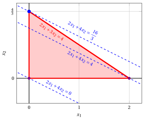
An optimal solution \({ \tilde{\boldsymbol x}}(\, LP\,)\) is:

\[ \tilde{x}_1=0,~~\tilde{x}_2=\dfrac{4}{3} \]

the optimal value \(z(\, LP\,)\) is \(\dfrac{16}{3}.\)

In violet the first and the second vertex explored by the previous execution of the revised simplex algorithm (before reaching the optimal one depicted in blue).

In dashed blue, the contour lines of the objective function associated with the values taken in the three vertices.

Exercise 11.2: Revised simplex algorithm (P1)

Consider the following LP problem in canonical maximization form with \(n=2\) variables and \(m=1\) constraint:

\[ \begin{array}{rrrrrr} {\max} & {x_1} & {+} & {8}\, {x_2} \\[2ex] \text{subject to} & {3}\, {x_1} & {+} & {6}\, {x_2} & {\le} & {16} \\[2ex] & {x_1,} & & {x_2} & {\ge} & {0} \end{array} \]

By introducing the slack variable, we get the following LP problem in standard maximization form with \(n+m=3\) variables and \(m=1\) constraint:

\[ \begin{array}{rrrrrrrr} {\max} & {x_1} & {+} & {8}\, {x_2} \\[2ex] \text{subject to} & {3}\, {x_1} & {+} & {6}\, {x_2} & {+} & {x_3} & {=} & {16} \\[2ex] & {x_1,} & & {x_2,} & & {x_3} & {\ge} & {0} \end{array} \]

Questions

• Execute the revised simplex algorithm to find an optimal solution of this LP problem using Bland's rule to select the pivot column and the pivot row.

Solution

We have:

\[ {\boldsymbol A}= \begin{pmatrix} 3 & 6 & 1 \end{pmatrix} \quad {\boldsymbol b}= \begin{pmatrix} 16 \end{pmatrix} \quad {\boldsymbol c}= \begin{pmatrix} 1\\ 8\\ 0 \end{pmatrix} \quad {\boldsymbol x}= \begin{pmatrix} x_1 \\ x_2 \\ x_3 \end{pmatrix} \]

• Initialization

  Since it is an LP problem in standard form obtained from an LP problem in canonical form with \(~{\boldsymbol b} \ge 0\) by adding the slack variables, the partition \(\pazocal{B}=\{3\}\) and \(\pazocal{N}=\{1,2\}\) is associated with the following basic feasible solution:

  \[ \begin{pmatrix} x_3 \end{pmatrix} = \begin{pmatrix} 16 \end{pmatrix} \text{ and } \begin{pmatrix} x_1 \\ x_2 \end{pmatrix} = \begin{pmatrix} 0\\ 0 \end{pmatrix} \]

• Iteration 1

  With \(\pazocal{B}= \{3\}\) and \(\pazocal{N}= \{1,~~2\}\), we have:

  \[ {\boldsymbol x}_{\pazocal{B}}= \begin{pmatrix} x_3 \end{pmatrix} ~~ {\boldsymbol A}_{\pazocal{B}}= \begin{pmatrix} 1 \end{pmatrix} ~~ {\boldsymbol c}_{\pazocal{B}}= \begin{pmatrix} 0 \end{pmatrix} ~~ {{ \bar{\boldsymbol b}}}= \begin{pmatrix} 16 \end{pmatrix} \]
  \[ {\boldsymbol x}_{\pazocal{N}}= \begin{pmatrix} x_1 \\ x_2 \end{pmatrix} ~~ {\boldsymbol A}_{\pazocal{N}}= \begin{pmatrix} 3 & 6 \end{pmatrix} ~~ {\boldsymbol c}_{\pazocal{N}}= \begin{pmatrix} 1\\ 8 \end{pmatrix} \]

  Optimality check

  We solve \({\boldsymbol \pi} \; {\boldsymbol A}_{\pazocal{B}} = {\boldsymbol c}'_{\pazocal{B}}\) to compute \({\boldsymbol \pi} = {{{\boldsymbol c}'_{\pazocal{B}} \; {\boldsymbol A}_{\pazocal{B}}^{-1}}}\), first system of linear equations:

  \[\begin{equation*} \begin{cases} \begin{array}{rrr} {\pi_3} & {=} & {0} \end{array} \end{cases} \qquad {\boldsymbol \pi}= \begin{pmatrix} 0\\ \end{pmatrix} \end{equation*}\]

  We compute the basic feasible solution value \({\bar{z}} = {\boldsymbol \pi} \; {\boldsymbol b} = \begin{pmatrix} 0\\ \end{pmatrix} \begin{pmatrix} 16 \end{pmatrix} = 0\)

  We compute the reduced costs \({{ \bar{\boldsymbol c}}'} = {{\boldsymbol c}'_{\pazocal{N}} - {\boldsymbol \pi} \; {\boldsymbol A}_{\pazocal{N}}}\):

  \[ {{ \bar{\boldsymbol c}}'} = \begin{pmatrix} 1 & 8\\ \end{pmatrix} - \begin{pmatrix} 0\\ \end{pmatrix} \begin{pmatrix} 3 & 6 \end{pmatrix} = \underbrace{ \begin{pmatrix} 1 & 8\\ \end{pmatrix} }_{{c_{1}~~~c_{2}}} - \underbrace{ \begin{pmatrix} 0 & 0\\ \end{pmatrix} }_{{\boldsymbol \pi}\;{\boldsymbol A}_{1} ~~{\boldsymbol \pi}\;{\boldsymbol A}_{2}} = \underbrace{ \begin{pmatrix} 1 & 8\\ \end{pmatrix} }_{{\bar{c}_{1}~~~\bar{c}_{2}}} \]

  Not all reduced costs are non-positive then we perform a pivoting operation.

  Pivoting operation

  Since \({c}_{1} > {\boldsymbol \pi} \;{\boldsymbol A}_{1}\), \(x_1\) is the pivot column and we have \({\boldsymbol A}_{1} = \begin{pmatrix} 3 \end{pmatrix}\)

  We solve \({\boldsymbol A}_{\pazocal{B}} \; {\boldsymbol d} = {\boldsymbol A}_{1}\) to compute \({\boldsymbol d}={ {\boldsymbol A}_{\pazocal{B}}^{-1}} {\boldsymbol A}_{1}\), second system of linear equations:

  \[\begin{equation*} \begin{cases} \begin{array}{rrr} {d_3} & {=} & {3} \end{array} \end{cases} \qquad {\boldsymbol d}= \begin{pmatrix} 3 \end{pmatrix} \end{equation*}\]

  We have to find the largest \(t\) such that \({{ \bar{\boldsymbol b}}} - t \; {{\boldsymbol d}} \ge 0\):

  \[ \begin{cases} \underbrace{16 -t \cdot 3\ge 0}_{x_3 \ge 0} \end{cases} \qquad \begin{cases} t\le \dfrac{16}{3} \end{cases} \text{ then } t_{m}=\dfrac{16}{3} \]

  Accordingly the value of the pivot column becomes \(t_{m}\), i.e., \(x_1=\dfrac{16}{3}\). The value of \(x_3\) becomes zero and \(x_3\) is the pivot row.

• Iteration 2

  With \(\pazocal{B}= \{1\}\) and \(\pazocal{N}= \{2,~~3\}\), we have:

  \[ {\boldsymbol x}_{\pazocal{B}}= \begin{pmatrix} x_1 \end{pmatrix} ~~ {\boldsymbol A}_{\pazocal{B}}= \begin{pmatrix} 3 \end{pmatrix} ~~ {\boldsymbol c}_{\pazocal{B}}= \begin{pmatrix} 1 \end{pmatrix} ~~ {{ \bar{\boldsymbol b}}}= \begin{pmatrix} \dfrac{16}{3} \end{pmatrix} \]
  \[ {\boldsymbol x}_{\pazocal{N}}= \begin{pmatrix} x_2 \\ x_3 \end{pmatrix} ~~ {\boldsymbol A}_{\pazocal{N}}= \begin{pmatrix} 6 & 1 \end{pmatrix} ~~ {\boldsymbol c}_{\pazocal{N}}= \begin{pmatrix} 8\\ 0 \end{pmatrix} \]

  Optimality check

  We solve \({\boldsymbol \pi} \; {\boldsymbol A}_{\pazocal{B}} = {\boldsymbol c}'_{\pazocal{B}}\) to compute \({\boldsymbol \pi} = {{{\boldsymbol c}'_{\pazocal{B}} \; {\boldsymbol A}_{\pazocal{B}}^{-1}}}\), first system of linear equations:

  \[\begin{equation*} \begin{cases} \begin{array}{rrr} {3}\, {\pi_1} & {=} & {1} \end{array} \end{cases} \qquad {\boldsymbol \pi}= \begin{pmatrix} \dfrac{1}{3}\\ \end{pmatrix} \end{equation*}\]

  We compute the basic feasible solution value \({\bar{z}} = {\boldsymbol \pi} \; {\boldsymbol b} = \begin{pmatrix} \dfrac{1}{3}\\ \end{pmatrix} \begin{pmatrix} 16 \end{pmatrix} = \dfrac{16}{3}\)

  We compute the reduced costs \({{ \bar{\boldsymbol c}}'} = {{\boldsymbol c}'_{\pazocal{N}} - {\boldsymbol \pi} \; {\boldsymbol A}_{\pazocal{N}}}\):

  \[ {{ \bar{\boldsymbol c}}'} = \begin{pmatrix} 8 & 0\\ \end{pmatrix} - \begin{pmatrix} \dfrac{1}{3}\\ \end{pmatrix} \begin{pmatrix} 6 & 1 \end{pmatrix} = \underbrace{ \begin{pmatrix} 8 & 0\\ \end{pmatrix} }_{{c_{2}~~~c_{3}}} - \underbrace{ \begin{pmatrix} 2 & \dfrac{1}{3}\\ \end{pmatrix} }_{{\boldsymbol \pi}\;{\boldsymbol A}_{2} ~~{\boldsymbol \pi}\;{\boldsymbol A}_{3}} = \underbrace{ \begin{pmatrix} 6 & -\dfrac{1}{3}\\ \end{pmatrix} }_{{\bar{c}_{2}~~~\bar{c}_{3}}} \]

  Not all reduced costs are non-positive then we perform a pivoting operation.

  Pivoting operation

  Since \({c}_{2} > {\boldsymbol \pi} \;{\boldsymbol A}_{2}\), \(x_2\) is the pivot column and we have \({\boldsymbol A}_{2} = \begin{pmatrix} 6 \end{pmatrix}\)

  We solve \({\boldsymbol A}_{\pazocal{B}} \; {\boldsymbol d} = {\boldsymbol A}_{2}\) to compute \({\boldsymbol d}={ {\boldsymbol A}_{\pazocal{B}}^{-1}} {\boldsymbol A}_{2}\), second system of linear equations:

  \[\begin{equation*} \begin{cases} \begin{array}{rrr} {3}\, {d_1} & {=} & {6} \end{array} \end{cases} \qquad {\boldsymbol d}= \begin{pmatrix} 2 \end{pmatrix} \end{equation*}\]

  We have to find the largest \(t\) such that \({{ \bar{\boldsymbol b}}} - t \; {{\boldsymbol d}} \ge 0\):

  \[ \begin{cases} \underbrace{\dfrac{16}{3} -t \cdot 2\ge 0}_{x_1 \ge 0} \end{cases} \qquad \begin{cases} t\le \dfrac{8}{3} \end{cases} \text{ then } t_{m}=\dfrac{8}{3} \]

  Accordingly the value of the pivot column becomes \(t_{m}\), i.e., \(x_2=\dfrac{8}{3}\). The value of \(x_1\) becomes zero and \(x_1\) is the pivot row.

• Iteration 3

  With \(\pazocal{B}= \{2\}\) and \(\pazocal{N}= \{1,~~3\}\), we have:

  \[ {\boldsymbol x}_{\pazocal{B}}= \begin{pmatrix} x_2 \end{pmatrix} ~~ {\boldsymbol A}_{\pazocal{B}}= \begin{pmatrix} 6 \end{pmatrix} ~~ {\boldsymbol c}_{\pazocal{B}}= \begin{pmatrix} 8 \end{pmatrix} ~~ {{ \bar{\boldsymbol b}}}= \begin{pmatrix} \dfrac{8}{3} \end{pmatrix} \]
  \[ {\boldsymbol x}_{\pazocal{N}}= \begin{pmatrix} x_1 \\ x_3 \end{pmatrix} ~~ {\boldsymbol A}_{\pazocal{N}}= \begin{pmatrix} 3 & 1 \end{pmatrix} ~~ {\boldsymbol c}_{\pazocal{N}}= \begin{pmatrix} 1\\ 0 \end{pmatrix} \]

  Optimality check

  We solve \({\boldsymbol \pi} \; {\boldsymbol A}_{\pazocal{B}} = {\boldsymbol c}'_{\pazocal{B}}\) to compute \({\boldsymbol \pi} = {{{\boldsymbol c}'_{\pazocal{B}} \; {\boldsymbol A}_{\pazocal{B}}^{-1}}}\), first system of linear equations:

  \[\begin{equation*} \begin{cases} \begin{array}{rrr} {6}\, {\pi_2} & {=} & {8} \end{array} \end{cases} \qquad {\boldsymbol \pi}= \begin{pmatrix} \dfrac{4}{3}\\ \end{pmatrix} \end{equation*}\]

  We compute the basic feasible solution value \({\bar{z}} = {\boldsymbol \pi} \; {\boldsymbol b} = \begin{pmatrix} \dfrac{4}{3}\\ \end{pmatrix} \begin{pmatrix} 16 \end{pmatrix} = \dfrac{64}{3}\)

  We compute the reduced costs \({{ \bar{\boldsymbol c}}'} = {{\boldsymbol c}'_{\pazocal{N}} - {\boldsymbol \pi} \; {\boldsymbol A}_{\pazocal{N}}}\):

  \[ {{ \bar{\boldsymbol c}}'} = \begin{pmatrix} 1 & 0\\ \end{pmatrix} - \begin{pmatrix} \dfrac{4}{3}\\ \end{pmatrix} \begin{pmatrix} 3 & 1 \end{pmatrix} = \underbrace{ \begin{pmatrix} 1 & 0\\ \end{pmatrix} }_{{c_{1}~~~c_{3}}} - \underbrace{ \begin{pmatrix} 4 & \dfrac{4}{3}\\ \end{pmatrix} }_{{\boldsymbol \pi}\;{\boldsymbol A}_{1} ~~{\boldsymbol \pi}\;{\boldsymbol A}_{3}} = \underbrace{ \begin{pmatrix} -3 & -\dfrac{4}{3}\\ \end{pmatrix} }_{{\bar{c}_{1}~~~\bar{c}_{3}}} \]

  All reduced costs are non-positive, then the basic feasible solution

  \[ {\boldsymbol x}_{\pazocal{B}}= \begin{pmatrix} x_2 \end{pmatrix}=\begin{pmatrix} \dfrac{8}{3} \end{pmatrix} \text{ and } {\boldsymbol x}_{\pazocal{N}}= \begin{pmatrix} x_1 \\ x_3 \end{pmatrix}=\begin{pmatrix} 0\\ 0 \end{pmatrix} \]

  is an optimal solution of the LP problem and \({\bar{z}} = \dfrac{64}{3}\) is the optimal solution value.

Graphical solution:

The feasible region of the LP problem (in canonical form) is the polyhedron shaded in red:

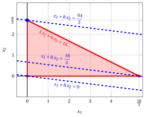
An optimal solution \({ \tilde{\boldsymbol x}}(\, LP\,)\) is:

\[ \tilde{x}_1=0,~~\tilde{x}_2=\dfrac{8}{3} \]

the optimal value \(z(\, LP\,)\) is \(\dfrac{64}{3}.\)

In violet the first and the second vertex explored by the previous execution of the revised simplex algorithm (before reaching the optimal one depicted in blue).

In dashed blue, the contour lines of the objective function associated with the values taken in the three vertices.

Exercise 11.3: Revised simplex algorithm (P2)

Consider the following LP problem in canonical maximization form with \(n=2\) variables and \(m=2\) constraints:

\[ \begin{array}{rrrrrr} {\max} & {x_1} & {+} & {3}\, {x_2} \\[2ex] \text{subject to} & {-4}\, {x_1} & {+} & {10}\, {x_2} & {\le} & {35} \\[2ex] & {3}\, {x_1} & {+} & {x_2} & {\le} & {12} \\[2ex] & {x_1,} & & {x_2} & {\ge} & {0} \end{array} \]

By introducing the slack variables, we get the following LP problem in standard maximization form with \(n+m=4\) variables and \(m=2\) constraints:

\[ \begin{array}{rrrrrrrrrr} {\max} & {x_1} & {+} & {3}\, {x_2} \\[2ex] \text{subject to} & {-4}\, {x_1} & {+} & {10}\, {x_2} & {+} & {x_3} & & & {=} & {35} \\[2ex] & {3}\, {x_1} & {+} & {x_2} & & & {+} & {x_4} & {=} & {12} \\[2ex] & {x_1,} & & {x_2,} & & {x_3,} & & {x_4} & {\ge} & {0} \end{array} \]

Questions

• Execute the revised simplex algorithm to find an optimal solution of this LP problem using Bland's rule to select the pivot column and the pivot row.

Solution

We have:

\[ {\boldsymbol A}= \begin{pmatrix} -4 & 10 & 1 & 0\\ 3 & 1 & 0 & 1 \end{pmatrix} \quad {\boldsymbol b}= \begin{pmatrix} 35\\ 12 \end{pmatrix} \quad {\boldsymbol c}= \begin{pmatrix} 1\\ 3\\ 0\\ 0 \end{pmatrix} \quad {\boldsymbol x}= \begin{pmatrix} x_1 \\ x_2 \\ x_3 \\ x_4 \end{pmatrix} \]

• Initialization

  Since it is an LP problem in standard form obtained from an LP problem in canonical form with \(~{\boldsymbol b} \ge 0\) by adding the slack variables, the partition \(\pazocal{B}=\{3,4\}\) and \(\pazocal{N}=\{1,2\}\) is associated with the following basic feasible solution:

  \[ \begin{pmatrix} x_3 \\ x_4 \end{pmatrix} = \begin{pmatrix} 35\\ 12 \end{pmatrix} \text{ and } \begin{pmatrix} x_1 \\ x_2 \end{pmatrix} = \begin{pmatrix} 0\\ 0 \end{pmatrix} \]

• Iteration 1

  With \(\pazocal{B}= \{3,~~4\}\) and \(\pazocal{N}= \{1,~~2\}\), we have:

  \[ {\boldsymbol x}_{\pazocal{B}}= \begin{pmatrix} x_3 \\ x_4 \end{pmatrix} ~~ {\boldsymbol A}_{\pazocal{B}}= \begin{pmatrix} 1 & 0\\ 0 & 1 \end{pmatrix} ~~ {\boldsymbol c}_{\pazocal{B}}= \begin{pmatrix} 0\\ 0 \end{pmatrix} ~~ {{ \bar{\boldsymbol b}}}= \begin{pmatrix} 35\\ 12 \end{pmatrix} \]
  \[ {\boldsymbol x}_{\pazocal{N}}= \begin{pmatrix} x_1 \\ x_2 \end{pmatrix} ~~ {\boldsymbol A}_{\pazocal{N}}= \begin{pmatrix} -4 & 10\\ 3 & 1 \end{pmatrix} ~~ {\boldsymbol c}_{\pazocal{N}}= \begin{pmatrix} 1\\ 3 \end{pmatrix} \]

  Optimality check

  We solve \({\boldsymbol \pi} \; {\boldsymbol A}_{\pazocal{B}} = {\boldsymbol c}'_{\pazocal{B}}\) to compute \({\boldsymbol \pi} = {{{\boldsymbol c}'_{\pazocal{B}} \; {\boldsymbol A}_{\pazocal{B}}^{-1}}}\), first system of linear equations:

  \[\begin{equation*} \begin{cases} \begin{array}{rrrrr} {\pi_3} & & & {=} & {0} \\[2ex] & & {\pi_4} & {=} & {0} \end{array} \end{cases} \qquad {\boldsymbol \pi}= \begin{pmatrix} 0 & 0\\ \end{pmatrix} \end{equation*}\]

  We compute the basic feasible solution value \({\bar{z}} = {\boldsymbol \pi} \; {\boldsymbol b} = \begin{pmatrix} 0 & 0\\ \end{pmatrix} \begin{pmatrix} 35\\ 12 \end{pmatrix} = 0\)

  We compute the reduced costs \({{ \bar{\boldsymbol c}}'} = {{\boldsymbol c}'_{\pazocal{N}} - {\boldsymbol \pi} \; {\boldsymbol A}_{\pazocal{N}}}\):

  \[ {{ \bar{\boldsymbol c}}'} = \begin{pmatrix} 1 & 3\\ \end{pmatrix} - \begin{pmatrix} 0 & 0\\ \end{pmatrix} \begin{pmatrix} -4 & 10\\ 3 & 1 \end{pmatrix} = \underbrace{ \begin{pmatrix} 1 & 3\\ \end{pmatrix} }_{{c_{1}~~~c_{2}}} - \underbrace{ \begin{pmatrix} 0 & 0\\ \end{pmatrix} }_{{\boldsymbol \pi}\;{\boldsymbol A}_{1} ~~{\boldsymbol \pi}\;{\boldsymbol A}_{2}} = \underbrace{ \begin{pmatrix} 1 & 3\\ \end{pmatrix} }_{{\bar{c}_{1}~~~\bar{c}_{2}}} \]

  Not all reduced costs are non-positive then we perform a pivoting operation.

  Pivoting operation

  Since \({c}_{1} > {\boldsymbol \pi} \;{\boldsymbol A}_{1}\), \(x_1\) is the pivot column and we have \({\boldsymbol A}_{1} = \begin{pmatrix} -4\\ 3 \end{pmatrix}\)

  We solve \({\boldsymbol A}_{\pazocal{B}} \; {\boldsymbol d} = {\boldsymbol A}_{1}\) to compute \({\boldsymbol d}={ {\boldsymbol A}_{\pazocal{B}}^{-1}} {\boldsymbol A}_{1}\), second system of linear equations:

  \[\begin{equation*} \begin{cases} \begin{array}{rrrrr} {d_3} & & & {=} & {-4} \\[2ex] & & {d_4} & {=} & {3} \end{array} \end{cases} \qquad {\boldsymbol d}= \begin{pmatrix} -4\\ 3 \end{pmatrix} \end{equation*}\]

  We have to find the largest \(t\) such that \({{ \bar{\boldsymbol b}}} - t \; {{\boldsymbol d}} \ge 0\):

  \[ \begin{cases} \underbrace{35 -t \cdot \left( -4\right)\ge 0}_{x_3 \ge 0} \\[2ex] \underbrace{12 -t \cdot 3\ge 0}_{x_4 \ge 0} \end{cases} \qquad \begin{cases} t\ge -\dfrac{35}{4} \\[2ex] t\le 4 \end{cases} \text{ then } t_{m}=4 \]

  Accordingly the value of the pivot column becomes \(t_{m}\), i.e., \(x_1=4\). The value of \(x_4\) becomes zero and \(x_4\) is the pivot row. The other basic variables take values \({ \bar{\boldsymbol b}} - t_{m} \; {\boldsymbol d}\), then we have:

  \[ x_3 = 35 - 4 \cdot \left( -4\right) = 51 \]

• Iteration 2

  With \(\pazocal{B}= \{1,~~3\}\) and \(\pazocal{N}= \{2,~~4\}\), we have:

  \[ {\boldsymbol x}_{\pazocal{B}}= \begin{pmatrix} x_1 \\ x_3 \end{pmatrix} ~~ {\boldsymbol A}_{\pazocal{B}}= \begin{pmatrix} -4 & 1\\ 3 & 0 \end{pmatrix} ~~ {\boldsymbol c}_{\pazocal{B}}= \begin{pmatrix} 1\\ 0 \end{pmatrix} ~~ {{ \bar{\boldsymbol b}}}= \begin{pmatrix} 4\\ 51 \end{pmatrix} \]
  \[ {\boldsymbol x}_{\pazocal{N}}= \begin{pmatrix} x_2 \\ x_4 \end{pmatrix} ~~ {\boldsymbol A}_{\pazocal{N}}= \begin{pmatrix} 10 & 0\\ 1 & 1 \end{pmatrix} ~~ {\boldsymbol c}_{\pazocal{N}}= \begin{pmatrix} 3\\ 0 \end{pmatrix} \]

  Optimality check

  We solve \({\boldsymbol \pi} \; {\boldsymbol A}_{\pazocal{B}} = {\boldsymbol c}'_{\pazocal{B}}\) to compute \({\boldsymbol \pi} = {{{\boldsymbol c}'_{\pazocal{B}} \; {\boldsymbol A}_{\pazocal{B}}^{-1}}}\), first system of linear equations:

  \[\begin{equation*} \begin{cases} \begin{array}{rrrrr} {-4}\, {\pi_1} & {+} & {3}\, {\pi_3} & {=} & {1} \\[2ex] {\pi_1} & & & {=} & {0} \end{array} \end{cases} \qquad {\boldsymbol \pi}= \begin{pmatrix} 0 & \dfrac{1}{3}\\ \end{pmatrix} \end{equation*}\]

  We compute the basic feasible solution value \({\bar{z}} = {\boldsymbol \pi} \; {\boldsymbol b} = \begin{pmatrix} 0 & \dfrac{1}{3}\\ \end{pmatrix} \begin{pmatrix} 35\\ 12 \end{pmatrix} = 4\)

  We compute the reduced costs \({{ \bar{\boldsymbol c}}'} = {{\boldsymbol c}'_{\pazocal{N}} - {\boldsymbol \pi} \; {\boldsymbol A}_{\pazocal{N}}}\):

  \[ {{ \bar{\boldsymbol c}}'} = \begin{pmatrix} 3 & 0\\ \end{pmatrix} - \begin{pmatrix} 0 & \dfrac{1}{3}\\ \end{pmatrix} \begin{pmatrix} 10 & 0\\ 1 & 1 \end{pmatrix} = \underbrace{ \begin{pmatrix} 3 & 0\\ \end{pmatrix} }_{{c_{2}~~~c_{4}}} - \underbrace{ \begin{pmatrix} \dfrac{1}{3} & \dfrac{1}{3}\\ \end{pmatrix} }_{{\boldsymbol \pi}\;{\boldsymbol A}_{2} ~~{\boldsymbol \pi}\;{\boldsymbol A}_{4}} = \underbrace{ \begin{pmatrix} \dfrac{8}{3} & -\dfrac{1}{3}\\ \end{pmatrix} }_{{\bar{c}_{2}~~~\bar{c}_{4}}} \]

  Not all reduced costs are non-positive then we perform a pivoting operation.

  Pivoting operation

  Since \({c}_{2} > {\boldsymbol \pi} \;{\boldsymbol A}_{2}\), \(x_2\) is the pivot column and we have \({\boldsymbol A}_{2} = \begin{pmatrix} 10\\ 1 \end{pmatrix}\)

  We solve \({\boldsymbol A}_{\pazocal{B}} \; {\boldsymbol d} = {\boldsymbol A}_{2}\) to compute \({\boldsymbol d}={ {\boldsymbol A}_{\pazocal{B}}^{-1}} {\boldsymbol A}_{2}\), second system of linear equations:

  \[\begin{equation*} \begin{cases} \begin{array}{rrrrr} {-4}\, {d_1} & {+} & {d_3} & {=} & {10} \\[2ex] {3}\, {d_1} & & & {=} & {1} \end{array} \end{cases} \qquad {\boldsymbol d}= \begin{pmatrix} \dfrac{1}{3}\\[2ex] \dfrac{34}{3} \end{pmatrix} \end{equation*}\]

  We have to find the largest \(t\) such that \({{ \bar{\boldsymbol b}}} - t \; {{\boldsymbol d}} \ge 0\):

  \[ \begin{cases} \underbrace{4 -t \cdot \dfrac{1}{3}\ge 0}_{x_1 \ge 0} \\[2ex] \underbrace{51 -t \cdot \dfrac{34}{3}\ge 0}_{x_3 \ge 0} \end{cases} \qquad \begin{cases} t\le 12 \\[2ex] t\le \dfrac{9}{2} \end{cases} \text{ then } t_{m}=\dfrac{9}{2} \]

  Accordingly the value of the pivot column becomes \(t_{m}\), i.e., \(x_2=\dfrac{9}{2}\). The value of \(x_3\) becomes zero and \(x_3\) is the pivot row. The other basic variables take values \({ \bar{\boldsymbol b}} - t_{m} \; {\boldsymbol d}\), then we have:

  \[ x_1 = 4 - \dfrac{9}{2} \cdot \dfrac{1}{3} = \dfrac{5}{2} \]

• Iteration 3

  With \(\pazocal{B}= \{1,~~2\}\) and \(\pazocal{N}= \{3,~~4\}\), we have:

  \[ {\boldsymbol x}_{\pazocal{B}}= \begin{pmatrix} x_1 \\ x_2 \end{pmatrix} ~~ {\boldsymbol A}_{\pazocal{B}}= \begin{pmatrix} -4 & 10\\ 3 & 1 \end{pmatrix} ~~ {\boldsymbol c}_{\pazocal{B}}= \begin{pmatrix} 1\\ 3 \end{pmatrix} ~~ {{ \bar{\boldsymbol b}}}= \begin{pmatrix} \dfrac{5}{2}\\[2ex] \dfrac{9}{2} \end{pmatrix} \]
  \[ {\boldsymbol x}_{\pazocal{N}}= \begin{pmatrix} x_3 \\ x_4 \end{pmatrix} ~~ {\boldsymbol A}_{\pazocal{N}}= \begin{pmatrix} 1 & 0\\ 0 & 1 \end{pmatrix} ~~ {\boldsymbol c}_{\pazocal{N}}= \begin{pmatrix} 0\\ 0 \end{pmatrix} \]

  Optimality check

  We solve \({\boldsymbol \pi} \; {\boldsymbol A}_{\pazocal{B}} = {\boldsymbol c}'_{\pazocal{B}}\) to compute \({\boldsymbol \pi} = {{{\boldsymbol c}'_{\pazocal{B}} \; {\boldsymbol A}_{\pazocal{B}}^{-1}}}\), first system of linear equations:

  \[\begin{equation*} \begin{cases} \begin{array}{rrrrr} {-4}\, {\pi_1} & {+} & {3}\, {\pi_2} & {=} & {1} \\[2ex] {10}\, {\pi_1} & {+} & {\pi_2} & {=} & {3} \end{array} \end{cases} \qquad {\boldsymbol \pi}= \begin{pmatrix} \dfrac{4}{17} & \dfrac{11}{17}\\ \end{pmatrix} \end{equation*}\]

  We compute the basic feasible solution value \({\bar{z}} = {\boldsymbol \pi} \; {\boldsymbol b} = \begin{pmatrix} \dfrac{4}{17} & \dfrac{11}{17}\\ \end{pmatrix} \begin{pmatrix} 35\\ 12 \end{pmatrix} = 16\)

  We compute the reduced costs \({{ \bar{\boldsymbol c}}'} = {{\boldsymbol c}'_{\pazocal{N}} - {\boldsymbol \pi} \; {\boldsymbol A}_{\pazocal{N}}}\):

  \[ {{ \bar{\boldsymbol c}}'} = \begin{pmatrix} 0 & 0\\ \end{pmatrix} - \begin{pmatrix} \dfrac{4}{17} & \dfrac{11}{17}\\ \end{pmatrix} \begin{pmatrix} 1 & 0\\ 0 & 1 \end{pmatrix} = \underbrace{ \begin{pmatrix} 0 & 0\\ \end{pmatrix} }_{{c_{3}~~~c_{4}}} - \underbrace{ \begin{pmatrix} \dfrac{4}{17} & \dfrac{11}{17}\\ \end{pmatrix} }_{{\boldsymbol \pi}\;{\boldsymbol A}_{3} ~~{\boldsymbol \pi}\;{\boldsymbol A}_{4}} = \underbrace{ \begin{pmatrix} -\dfrac{4}{17} & -\dfrac{11}{17}\\ \end{pmatrix} }_{{\bar{c}_{3}~~~\bar{c}_{4}}} \]

  All reduced costs are non-positive, then the basic feasible solution

  \[ {\boldsymbol x}_{\pazocal{B}}= \begin{pmatrix} x_1 \\ x_2 \end{pmatrix}=\begin{pmatrix} \dfrac{5}{2}\\[2ex] \dfrac{9}{2} \end{pmatrix} \text{ and } {\boldsymbol x}_{\pazocal{N}}= \begin{pmatrix} x_3 \\ x_4 \end{pmatrix}=\begin{pmatrix} 0\\ 0 \end{pmatrix} \]

  is an optimal solution of the LP problem and \({\bar{z}} = 16\) is the optimal solution value.

Graphical solution:

The feasible region of the LP problem (in canonical form) is the polyhedron shaded in red:

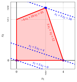
An optimal solution \({ \tilde{\boldsymbol x}}(\, LP\,)\) is:

\[ \tilde{x}_1=\dfrac{5}{2},~~\tilde{x}_2=\dfrac{9}{2} \]

the optimal value \(z(\, LP\,)\) is \(16.\)

In violet the first and the second vertex explored by the previous execution of the revised simplex algorithm (before reaching the optimal one depicted in blue).

In dashed blue, the contour lines of the objective function associated with the values taken in the three vertices.

Exercise 11.4: Revised simplex algorithm (P3)

Consider the following LP problem in canonical maximization form with \(n=2\) variables and \(m=2\) constraints:

\[ \begin{array}{rrrrrr} {\max} & {2}\, {x_1} & {+} & {4}\, {x_2} \\[2ex] \text{subject to} & {-x_1} & {+} & {x_2} & {\le} & {2} \\[2ex] & {8}\, {x_1} & {+} & {2}\, {x_2} & {\le} & {19} \\[2ex] & {x_1,} & & {x_2} & {\ge} & {0} \end{array} \]

By introducing the slack variables, we get the following LP problem in standard maximization form with \(n+m=4\) variables and \(m=2\) constraints:

\[ \begin{array}{rrrrrrrrrr} {\max} & {2}\, {x_1} & {+} & {4}\, {x_2} \\[2ex] \text{subject to} & {-x_1} & {+} & {x_2} & {+} & {x_3} & & & {=} & {2} \\[2ex] & {8}\, {x_1} & {+} & {2}\, {x_2} & & & {+} & {x_4} & {=} & {19} \\[2ex] & {x_1,} & & {x_2,} & & {x_3,} & & {x_4} & {\ge} & {0} \end{array} \]

Questions

• Execute the revised simplex algorithm to find an optimal solution of this LP problem using Bland's rule to select the pivot column and the pivot row.

Solution

We have:

\[ {\boldsymbol A}= \begin{pmatrix} -1 & 1 & 1 & 0\\ 8 & 2 & 0 & 1 \end{pmatrix} \quad {\boldsymbol b}= \begin{pmatrix} 2\\ 19 \end{pmatrix} \quad {\boldsymbol c}= \begin{pmatrix} 2\\ 4\\ 0\\ 0 \end{pmatrix} \quad {\boldsymbol x}= \begin{pmatrix} x_1 \\ x_2 \\ x_3 \\ x_4 \end{pmatrix} \]

• Initialization

  Since it is an LP problem in standard form obtained from an LP problem in canonical form with \(~{\boldsymbol b} \ge 0\) by adding the slack variables, the partition \(\pazocal{B}=\{3,4\}\) and \(\pazocal{N}=\{1,2\}\) is associated with the following basic feasible solution:

  \[ \begin{pmatrix} x_3 \\ x_4 \end{pmatrix} = \begin{pmatrix} 2\\ 19 \end{pmatrix} \text{ and } \begin{pmatrix} x_1 \\ x_2 \end{pmatrix} = \begin{pmatrix} 0\\ 0 \end{pmatrix} \]

• Iteration 1

  With \(\pazocal{B}= \{3,~~4\}\) and \(\pazocal{N}= \{1,~~2\}\), we have:

  \[ {\boldsymbol x}_{\pazocal{B}}= \begin{pmatrix} x_3 \\ x_4 \end{pmatrix} ~~ {\boldsymbol A}_{\pazocal{B}}= \begin{pmatrix} 1 & 0\\ 0 & 1 \end{pmatrix} ~~ {\boldsymbol c}_{\pazocal{B}}= \begin{pmatrix} 0\\ 0 \end{pmatrix} ~~ {{ \bar{\boldsymbol b}}}= \begin{pmatrix} 2\\ 19 \end{pmatrix} \]
  \[ {\boldsymbol x}_{\pazocal{N}}= \begin{pmatrix} x_1 \\ x_2 \end{pmatrix} ~~ {\boldsymbol A}_{\pazocal{N}}= \begin{pmatrix} -1 & 1\\ 8 & 2 \end{pmatrix} ~~ {\boldsymbol c}_{\pazocal{N}}= \begin{pmatrix} 2\\ 4 \end{pmatrix} \]

  Optimality check

  We solve \({\boldsymbol \pi} \; {\boldsymbol A}_{\pazocal{B}} = {\boldsymbol c}'_{\pazocal{B}}\) to compute \({\boldsymbol \pi} = {{{\boldsymbol c}'_{\pazocal{B}} \; {\boldsymbol A}_{\pazocal{B}}^{-1}}}\), first system of linear equations:

  \[\begin{equation*} \begin{cases} \begin{array}{rrrrr} {\pi_3} & & & {=} & {0} \\[2ex] & & {\pi_4} & {=} & {0} \end{array} \end{cases} \qquad {\boldsymbol \pi}= \begin{pmatrix} 0 & 0\\ \end{pmatrix} \end{equation*}\]

  We compute the basic feasible solution value \({\bar{z}} = {\boldsymbol \pi} \; {\boldsymbol b} = \begin{pmatrix} 0 & 0\\ \end{pmatrix} \begin{pmatrix} 2\\ 19 \end{pmatrix} = 0\)

  We compute the reduced costs \({{ \bar{\boldsymbol c}}'} = {{\boldsymbol c}'_{\pazocal{N}} - {\boldsymbol \pi} \; {\boldsymbol A}_{\pazocal{N}}}\):

  \[ {{ \bar{\boldsymbol c}}'} = \begin{pmatrix} 2 & 4\\ \end{pmatrix} - \begin{pmatrix} 0 & 0\\ \end{pmatrix} \begin{pmatrix} -1 & 1\\ 8 & 2 \end{pmatrix} = \underbrace{ \begin{pmatrix} 2 & 4\\ \end{pmatrix} }_{{c_{1}~~~c_{2}}} - \underbrace{ \begin{pmatrix} 0 & 0\\ \end{pmatrix} }_{{\boldsymbol \pi}\;{\boldsymbol A}_{1} ~~{\boldsymbol \pi}\;{\boldsymbol A}_{2}} = \underbrace{ \begin{pmatrix} 2 & 4\\ \end{pmatrix} }_{{\bar{c}_{1}~~~\bar{c}_{2}}} \]

  Not all reduced costs are non-positive then we perform a pivoting operation.

  Pivoting operation

  Since \({c}_{1} > {\boldsymbol \pi} \;{\boldsymbol A}_{1}\), \(x_1\) is the pivot column and we have \({\boldsymbol A}_{1} = \begin{pmatrix} -1\\ 8 \end{pmatrix}\)

  We solve \({\boldsymbol A}_{\pazocal{B}} \; {\boldsymbol d} = {\boldsymbol A}_{1}\) to compute \({\boldsymbol d}={ {\boldsymbol A}_{\pazocal{B}}^{-1}} {\boldsymbol A}_{1}\), second system of linear equations:

  \[\begin{equation*} \begin{cases} \begin{array}{rrrrr} {d_3} & & & {=} & {-1} \\[2ex] & & {d_4} & {=} & {8} \end{array} \end{cases} \qquad {\boldsymbol d}= \begin{pmatrix} -1\\ 8 \end{pmatrix} \end{equation*}\]

  We have to find the largest \(t\) such that \({{ \bar{\boldsymbol b}}} - t \; {{\boldsymbol d}} \ge 0\):

  \[ \begin{cases} \underbrace{2 -t \cdot \left( -1\right)\ge 0}_{x_3 \ge 0} \\[2ex] \underbrace{19 -t \cdot 8\ge 0}_{x_4 \ge 0} \end{cases} \qquad \begin{cases} t\ge -2 \\[2ex] t\le \dfrac{19}{8} \end{cases} \text{ then } t_{m}=\dfrac{19}{8} \]

  Accordingly the value of the pivot column becomes \(t_{m}\), i.e., \(x_1=\dfrac{19}{8}\). The value of \(x_4\) becomes zero and \(x_4\) is the pivot row. The other basic variables take values \({ \bar{\boldsymbol b}} - t_{m} \; {\boldsymbol d}\), then we have:

  \[ x_3 = 2 - \dfrac{19}{8} \cdot \left( -1\right) = \dfrac{35}{8} \]

• Iteration 2

  With \(\pazocal{B}= \{1,~~3\}\) and \(\pazocal{N}= \{2,~~4\}\), we have:

  \[ {\boldsymbol x}_{\pazocal{B}}= \begin{pmatrix} x_1 \\ x_3 \end{pmatrix} ~~ {\boldsymbol A}_{\pazocal{B}}= \begin{pmatrix} -1 & 1\\ 8 & 0 \end{pmatrix} ~~ {\boldsymbol c}_{\pazocal{B}}= \begin{pmatrix} 2\\ 0 \end{pmatrix} ~~ {{ \bar{\boldsymbol b}}}= \begin{pmatrix} \dfrac{19}{8}\\[2ex] \dfrac{35}{8} \end{pmatrix} \]
  \[ {\boldsymbol x}_{\pazocal{N}}= \begin{pmatrix} x_2 \\ x_4 \end{pmatrix} ~~ {\boldsymbol A}_{\pazocal{N}}= \begin{pmatrix} 1 & 0\\ 2 & 1 \end{pmatrix} ~~ {\boldsymbol c}_{\pazocal{N}}= \begin{pmatrix} 4\\ 0 \end{pmatrix} \]

  Optimality check

  We solve \({\boldsymbol \pi} \; {\boldsymbol A}_{\pazocal{B}} = {\boldsymbol c}'_{\pazocal{B}}\) to compute \({\boldsymbol \pi} = {{{\boldsymbol c}'_{\pazocal{B}} \; {\boldsymbol A}_{\pazocal{B}}^{-1}}}\), first system of linear equations:

  \[\begin{equation*} \begin{cases} \begin{array}{rrrrr} {-\pi_1} & {+} & {8}\, {\pi_3} & {=} & {2} \\[2ex] {\pi_1} & & & {=} & {0} \end{array} \end{cases} \qquad {\boldsymbol \pi}= \begin{pmatrix} 0 & \dfrac{1}{4}\\ \end{pmatrix} \end{equation*}\]

  We compute the basic feasible solution value \({\bar{z}} = {\boldsymbol \pi} \; {\boldsymbol b} = \begin{pmatrix} 0 & \dfrac{1}{4}\\ \end{pmatrix} \begin{pmatrix} 2\\ 19 \end{pmatrix} = \dfrac{19}{4}\)

  We compute the reduced costs \({{ \bar{\boldsymbol c}}'} = {{\boldsymbol c}'_{\pazocal{N}} - {\boldsymbol \pi} \; {\boldsymbol A}_{\pazocal{N}}}\):

  \[ {{ \bar{\boldsymbol c}}'} = \begin{pmatrix} 4 & 0\\ \end{pmatrix} - \begin{pmatrix} 0 & \dfrac{1}{4}\\ \end{pmatrix} \begin{pmatrix} 1 & 0\\ 2 & 1 \end{pmatrix} = \underbrace{ \begin{pmatrix} 4 & 0\\ \end{pmatrix} }_{{c_{2}~~~c_{4}}} - \underbrace{ \begin{pmatrix} \dfrac{1}{2} & \dfrac{1}{4}\\ \end{pmatrix} }_{{\boldsymbol \pi}\;{\boldsymbol A}_{2} ~~{\boldsymbol \pi}\;{\boldsymbol A}_{4}} = \underbrace{ \begin{pmatrix} \dfrac{7}{2} & -\dfrac{1}{4}\\ \end{pmatrix} }_{{\bar{c}_{2}~~~\bar{c}_{4}}} \]

  Not all reduced costs are non-positive then we perform a pivoting operation.

  Pivoting operation

  Since \({c}_{2} > {\boldsymbol \pi} \;{\boldsymbol A}_{2}\), \(x_2\) is the pivot column and we have \({\boldsymbol A}_{2} = \begin{pmatrix} 1\\ 2 \end{pmatrix}\)

  We solve \({\boldsymbol A}_{\pazocal{B}} \; {\boldsymbol d} = {\boldsymbol A}_{2}\) to compute \({\boldsymbol d}={ {\boldsymbol A}_{\pazocal{B}}^{-1}} {\boldsymbol A}_{2}\), second system of linear equations:

  \[\begin{equation*} \begin{cases} \begin{array}{rrrrr} {-d_1} & {+} & {d_3} & {=} & {1} \\[2ex] {8}\, {d_1} & & & {=} & {2} \end{array} \end{cases} \qquad {\boldsymbol d}= \begin{pmatrix} \dfrac{1}{4}\\[2ex] \dfrac{5}{4} \end{pmatrix} \end{equation*}\]

  We have to find the largest \(t\) such that \({{ \bar{\boldsymbol b}}} - t \; {{\boldsymbol d}} \ge 0\):

  \[ \begin{cases} \underbrace{\dfrac{19}{8} -t \cdot \dfrac{1}{4}\ge 0}_{x_1 \ge 0} \\[2ex] \underbrace{\dfrac{35}{8} -t \cdot \dfrac{5}{4}\ge 0}_{x_3 \ge 0} \end{cases} \qquad \begin{cases} t\le \dfrac{19}{2} \\[2ex] t\le \dfrac{7}{2} \end{cases} \text{ then } t_{m}=\dfrac{7}{2} \]

  Accordingly the value of the pivot column becomes \(t_{m}\), i.e., \(x_2=\dfrac{7}{2}\). The value of \(x_3\) becomes zero and \(x_3\) is the pivot row. The other basic variables take values \({ \bar{\boldsymbol b}} - t_{m} \; {\boldsymbol d}\), then we have:

  \[ x_1 = \dfrac{19}{8} - \dfrac{7}{2} \cdot \dfrac{1}{4} = \dfrac{3}{2} \]

• Iteration 3

  With \(\pazocal{B}= \{1,~~2\}\) and \(\pazocal{N}= \{3,~~4\}\), we have:

  \[ {\boldsymbol x}_{\pazocal{B}}= \begin{pmatrix} x_1 \\ x_2 \end{pmatrix} ~~ {\boldsymbol A}_{\pazocal{B}}= \begin{pmatrix} -1 & 1\\ 8 & 2 \end{pmatrix} ~~ {\boldsymbol c}_{\pazocal{B}}= \begin{pmatrix} 2\\ 4 \end{pmatrix} ~~ {{ \bar{\boldsymbol b}}}= \begin{pmatrix} \dfrac{3}{2}\\[2ex] \dfrac{7}{2} \end{pmatrix} \]
  \[ {\boldsymbol x}_{\pazocal{N}}= \begin{pmatrix} x_3 \\ x_4 \end{pmatrix} ~~ {\boldsymbol A}_{\pazocal{N}}= \begin{pmatrix} 1 & 0\\ 0 & 1 \end{pmatrix} ~~ {\boldsymbol c}_{\pazocal{N}}= \begin{pmatrix} 0\\ 0 \end{pmatrix} \]

  Optimality check

  We solve \({\boldsymbol \pi} \; {\boldsymbol A}_{\pazocal{B}} = {\boldsymbol c}'_{\pazocal{B}}\) to compute \({\boldsymbol \pi} = {{{\boldsymbol c}'_{\pazocal{B}} \; {\boldsymbol A}_{\pazocal{B}}^{-1}}}\), first system of linear equations:

  \[\begin{equation*} \begin{cases} \begin{array}{rrrrr} {-\pi_1} & {+} & {8}\, {\pi_2} & {=} & {2} \\[2ex] {\pi_1} & {+} & {2}\, {\pi_2} & {=} & {4} \end{array} \end{cases} \qquad {\boldsymbol \pi}= \begin{pmatrix} \dfrac{14}{5} & \dfrac{3}{5}\\ \end{pmatrix} \end{equation*}\]

  We compute the basic feasible solution value \({\bar{z}} = {\boldsymbol \pi} \; {\boldsymbol b} = \begin{pmatrix} \dfrac{14}{5} & \dfrac{3}{5}\\ \end{pmatrix} \begin{pmatrix} 2\\ 19 \end{pmatrix} = 17\)

  We compute the reduced costs \({{ \bar{\boldsymbol c}}'} = {{\boldsymbol c}'_{\pazocal{N}} - {\boldsymbol \pi} \; {\boldsymbol A}_{\pazocal{N}}}\):

  \[ {{ \bar{\boldsymbol c}}'} = \begin{pmatrix} 0 & 0\\ \end{pmatrix} - \begin{pmatrix} \dfrac{14}{5} & \dfrac{3}{5}\\ \end{pmatrix} \begin{pmatrix} 1 & 0\\ 0 & 1 \end{pmatrix} = \underbrace{ \begin{pmatrix} 0 & 0\\ \end{pmatrix} }_{{c_{3}~~~c_{4}}} - \underbrace{ \begin{pmatrix} \dfrac{14}{5} & \dfrac{3}{5}\\ \end{pmatrix} }_{{\boldsymbol \pi}\;{\boldsymbol A}_{3} ~~{\boldsymbol \pi}\;{\boldsymbol A}_{4}} = \underbrace{ \begin{pmatrix} -\dfrac{14}{5} & -\dfrac{3}{5}\\ \end{pmatrix} }_{{\bar{c}_{3}~~~\bar{c}_{4}}} \]

  All reduced costs are non-positive, then the basic feasible solution

  \[ {\boldsymbol x}_{\pazocal{B}}= \begin{pmatrix} x_1 \\ x_2 \end{pmatrix}=\begin{pmatrix} \dfrac{3}{2}\\[2ex] \dfrac{7}{2} \end{pmatrix} \text{ and } {\boldsymbol x}_{\pazocal{N}}= \begin{pmatrix} x_3 \\ x_4 \end{pmatrix}=\begin{pmatrix} 0\\ 0 \end{pmatrix} \]

  is an optimal solution of the LP problem and \({\bar{z}} = 17\) is the optimal solution value.

Graphical solution:

The feasible region of the LP problem (in canonical form) is the polyhedron shaded in red:

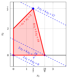
An optimal solution \({ \tilde{\boldsymbol x}}(\, LP \,)\) is:

\[ \tilde{x}_1=\dfrac{3}{2},~~\tilde{x}_2=\dfrac{7}{2} \]

the optimal value \(z(\, LP\,)\) is \(17.\)

In violet the first and the second vertex explored by the previous execution of the revised simplex algorithm (before reaching the optimal one depicted in blue).

In dashed blue, the contour lines of the objective function associated with the values taken in the three vertices.

Exercise 11.5: Revised simplex algorithm (P4)

Consider the following LP problem in canonical maximization form with \(n=2\) variables and \(m=2\) constraints:

\[ \begin{array}{rrrrrr} {\max} & {5}\, {x_1} & {+} & {3}\, {x_2} \\[2ex] \text{subject to} & {2}\, {x_1} & {+} & {x_2} & {\le} & {14} \\[2ex] & {x_1} & {+} & {8}\, {x_2} & {\le} & {32} \\[2ex] & {x_1,} & & {x_2} & {\ge} & {0} \end{array} \]

By introducing the slack variables, we get the following LP problem in standard maximization form with \(n+m=4\) variables and \(m=2\) constraints:

\[ \begin{array}{rrrrrrrrrr} {\max} & {5}\, {x_1} & {+} & {3}\, {x_2} \\[2ex] \text{subject to} & {2}\, {x_1} & {+} & {x_2} & {+} & {x_3} & & & {=} & {14} \\[2ex] & {x_1} & {+} & {8}\, {x_2} & & & {+} & {x_4} & {=} & {32} \\[2ex] & {x_1,} & & {x_2,} & & {x_3,} & & {x_4} & {\ge} & {0} \end{array} \]

Questions

• Execute the revised simplex algorithm to find an optimal solution of this LP problem using Bland's rule to select the pivot column and the pivot row.

Solution

We have:

\[ {\boldsymbol A}= \begin{pmatrix} 2 & 1 & 1 & 0\\ 1 & 8 & 0 & 1 \end{pmatrix} \quad {\boldsymbol b}= \begin{pmatrix} 14\\ 32 \end{pmatrix} \quad {\boldsymbol c}= \begin{pmatrix} 5\\ 3\\ 0\\ 0 \end{pmatrix} \quad {\boldsymbol x}= \begin{pmatrix} x_1 \\ x_2 \\ x_3 \\ x_4 \end{pmatrix} \]

• Initialization

  Since it is an LP problem in standard form obtained from an LP problem in canonical form with \(~{\boldsymbol b} \ge 0\) by adding the slack variables, the partition \(\pazocal{B}=\{3,4\}\) and \(\pazocal{N}=\{1,2\}\) is associated with the following basic feasible solution:

  \[ \begin{pmatrix} x_3 \\ x_4 \end{pmatrix} = \begin{pmatrix} 14\\ 32 \end{pmatrix} \text{ and } \begin{pmatrix} x_1 \\ x_2 \end{pmatrix} = \begin{pmatrix} 0\\ 0 \end{pmatrix} \]

• Iteration 1

  With \(\pazocal{B}= \{3,~~4\}\) and \(\pazocal{N}= \{1,~~2\}\), we have:

  \[ {\boldsymbol x}_{\pazocal{B}}= \begin{pmatrix} x_3 \\ x_4 \end{pmatrix} ~~ {\boldsymbol A}_{\pazocal{B}}= \begin{pmatrix} 1 & 0\\ 0 & 1 \end{pmatrix} ~~ {\boldsymbol c}_{\pazocal{B}}= \begin{pmatrix} 0\\ 0 \end{pmatrix} ~~ {{ \bar{\boldsymbol b}}}= \begin{pmatrix} 14\\ 32 \end{pmatrix} \]
  \[ {\boldsymbol x}_{\pazocal{N}}= \begin{pmatrix} x_1 \\ x_2 \end{pmatrix} ~~ {\boldsymbol A}_{\pazocal{N}}= \begin{pmatrix} 2 & 1\\ 1 & 8 \end{pmatrix} ~~ {\boldsymbol c}_{\pazocal{N}}= \begin{pmatrix} 5\\ 3 \end{pmatrix} \]

  Optimality check

  We solve \({\boldsymbol \pi} \; {\boldsymbol A}_{\pazocal{B}} = {\boldsymbol c}'_{\pazocal{B}}\) to compute \({\boldsymbol \pi} = {{{\boldsymbol c}'_{\pazocal{B}} \; {\boldsymbol A}_{\pazocal{B}}^{-1}}}\), first system of linear equations:

  \[\begin{equation*} \begin{cases} \begin{array}{rrrrr} {\pi_3} & & & {=} & {0} \\[2ex] & & {\pi_4} & {=} & {0} \end{array} \end{cases} \qquad {\boldsymbol \pi}= \begin{pmatrix} 0 & 0\\ \end{pmatrix} \end{equation*}\]

  We compute the basic feasible solution value \({\bar{z}} = {\boldsymbol \pi} \; {\boldsymbol b} = \begin{pmatrix} 0 & 0\\ \end{pmatrix} \begin{pmatrix} 14\\ 32 \end{pmatrix} = 0\)

  We compute the reduced costs \({{ \bar{\boldsymbol c}}'} = {{\boldsymbol c}'_{\pazocal{N}} - {\boldsymbol \pi} \; {\boldsymbol A}_{\pazocal{N}}}\):

  \[ {{ \bar{\boldsymbol c}}'} = \begin{pmatrix} 5 & 3\\ \end{pmatrix} - \begin{pmatrix} 0 & 0\\ \end{pmatrix} \begin{pmatrix} 2 & 1\\ 1 & 8 \end{pmatrix} = \underbrace{ \begin{pmatrix} 5 & 3\\ \end{pmatrix} }_{{c_{1}~~~c_{2}}} - \underbrace{ \begin{pmatrix} 0 & 0\\ \end{pmatrix} }_{{\boldsymbol \pi}\;{\boldsymbol A}_{1} ~~{\boldsymbol \pi}\;{\boldsymbol A}_{2}} = \underbrace{ \begin{pmatrix} 5 & 3\\ \end{pmatrix} }_{{\bar{c}_{1}~~~\bar{c}_{2}}} \]

  Not all reduced costs are non-positive then we perform a pivoting operation.

  Pivoting operation

  Since \({c}_{1} > {\boldsymbol \pi} \;{\boldsymbol A}_{1}\), \(x_1\) is the pivot column and we have \({\boldsymbol A}_{1} = \begin{pmatrix} 2\\ 1 \end{pmatrix}\)

  We solve \({\boldsymbol A}_{\pazocal{B}} \; {\boldsymbol d} = {\boldsymbol A}_{1}\) to compute \({\boldsymbol d}={ {\boldsymbol A}_{\pazocal{B}}^{-1}} {\boldsymbol A}_{1}\), second system of linear equations:

  \[\begin{equation*} \begin{cases} \begin{array}{rrrrr} {d_3} & & & {=} & {2} \\[2ex] & & {d_4} & {=} & {1} \end{array} \end{cases} \qquad {\boldsymbol d}= \begin{pmatrix} 2\\ 1 \end{pmatrix} \end{equation*}\]

  We have to find the largest \(t\) such that \({{ \bar{\boldsymbol b}}} - t \; {{\boldsymbol d}} \ge 0\):

  \[ \begin{cases} \underbrace{14 -t \cdot 2\ge 0}_{x_3 \ge 0} \\[2ex] \underbrace{32 -t \cdot 1\ge 0}_{x_4 \ge 0} \end{cases} \qquad \begin{cases} t\le 7 \\[2ex] t\le 32 \end{cases} \text{ then } t_{m}=7 \]

  Accordingly the value of the pivot column becomes \(t_{m}\), i.e., \(x_1=7\). The value of \(x_3\) becomes zero and \(x_3\) is the pivot row. The other basic variables take values \({ \bar{\boldsymbol b}} - t_{m} \; {\boldsymbol d}\), then we have:

  \[ x_4 = 32 - 7 \cdot 1 = 25 \]

• Iteration 2

  With \(\pazocal{B}= \{1,~~4\}\) and \(\pazocal{N}= \{2,~~3\}\), we have:

  \[ {\boldsymbol x}_{\pazocal{B}}= \begin{pmatrix} x_1 \\ x_4 \end{pmatrix} ~~ {\boldsymbol A}_{\pazocal{B}}= \begin{pmatrix} 2 & 0\\ 1 & 1 \end{pmatrix} ~~ {\boldsymbol c}_{\pazocal{B}}= \begin{pmatrix} 5\\ 0 \end{pmatrix} ~~ {{ \bar{\boldsymbol b}}}= \begin{pmatrix} 7\\ 25 \end{pmatrix} \]
  \[ {\boldsymbol x}_{\pazocal{N}}= \begin{pmatrix} x_2 \\ x_3 \end{pmatrix} ~~ {\boldsymbol A}_{\pazocal{N}}= \begin{pmatrix} 1 & 1\\ 8 & 0 \end{pmatrix} ~~ {\boldsymbol c}_{\pazocal{N}}= \begin{pmatrix} 3\\ 0 \end{pmatrix} \]

  Optimality check

  We solve \({\boldsymbol \pi} \; {\boldsymbol A}_{\pazocal{B}} = {\boldsymbol c}'_{\pazocal{B}}\) to compute \({\boldsymbol \pi} = {{{\boldsymbol c}'_{\pazocal{B}} \; {\boldsymbol A}_{\pazocal{B}}^{-1}}}\), first system of linear equations:

  \[\begin{equation*} \begin{cases} \begin{array}{rrrrr} {2}\, {\pi_1} & {+} & {\pi_4} & {=} & {5} \\[2ex] & & {\pi_4} & {=} & {0} \end{array} \end{cases} \qquad {\boldsymbol \pi}= \begin{pmatrix} \dfrac{5}{2} & 0\\ \end{pmatrix} \end{equation*}\]

  We compute the basic feasible solution value \({\bar{z}} = {\boldsymbol \pi} \; {\boldsymbol b} = \begin{pmatrix} \dfrac{5}{2} & 0\\ \end{pmatrix} \begin{pmatrix} 14\\ 32 \end{pmatrix} = 35\)

  We compute the reduced costs \({{ \bar{\boldsymbol c}}'} = {{\boldsymbol c}'_{\pazocal{N}} - {\boldsymbol \pi} \; {\boldsymbol A}_{\pazocal{N}}}\):

  \[ {{ \bar{\boldsymbol c}}'} = \begin{pmatrix} 3 & 0\\ \end{pmatrix} - \begin{pmatrix} \dfrac{5}{2} & 0\\ \end{pmatrix} \begin{pmatrix} 1 & 1\\ 8 & 0 \end{pmatrix} = \underbrace{ \begin{pmatrix} 3 & 0\\ \end{pmatrix} }_{{c_{2}~~~c_{3}}} - \underbrace{ \begin{pmatrix} \dfrac{5}{2} & \dfrac{5}{2}\\ \end{pmatrix} }_{{\boldsymbol \pi}\;{\boldsymbol A}_{2} ~~{\boldsymbol \pi}\;{\boldsymbol A}_{3}} = \underbrace{ \begin{pmatrix} \dfrac{1}{2} & -\dfrac{5}{2}\\ \end{pmatrix} }_{{\bar{c}_{2}~~~\bar{c}_{3}}} \]

  Not all reduced costs are non-positive then we perform a pivoting operation.

  Pivoting operation

  Since \({c}_{2} > {\boldsymbol \pi} \;{\boldsymbol A}_{2}\), \(x_2\) is the pivot column and we have \({\boldsymbol A}_{2} = \begin{pmatrix} 1\\ 8 \end{pmatrix}\)

  We solve \({\boldsymbol A}_{\pazocal{B}} \; {\boldsymbol d} = {\boldsymbol A}_{2}\) to compute \({\boldsymbol d}={ {\boldsymbol A}_{\pazocal{B}}^{-1}} {\boldsymbol A}_{2}\), second system of linear equations:

  \[\begin{equation*} \begin{cases} \begin{array}{rrrrr} {2}\, {d_1} & & & {=} & {1} \\[2ex] {d_1} & {+} & {d_4} & {=} & {8} \end{array} \end{cases} \qquad {\boldsymbol d}= \begin{pmatrix} \dfrac{1}{2}\\[2ex] \dfrac{15}{2} \end{pmatrix} \end{equation*}\]

  We have to find the largest \(t\) such that \({{ \bar{\boldsymbol b}}} - t \; {{\boldsymbol d}} \ge 0\):

  \[ \begin{cases} \underbrace{7 -t \cdot \dfrac{1}{2}\ge 0}_{x_1 \ge 0} \\[2ex] \underbrace{25 -t \cdot \dfrac{15}{2}\ge 0}_{x_4 \ge 0} \end{cases} \qquad \begin{cases} t\le 14 \\[2ex] t\le \dfrac{10}{3} \end{cases} \text{ then } t_{m}=\dfrac{10}{3} \]

  Accordingly the value of the pivot column becomes \(t_{m}\), i.e., \(x_2=\dfrac{10}{3}\). The value of \(x_4\) becomes zero and \(x_4\) is the pivot row. The other basic variables take values \({ \bar{\boldsymbol b}} - t_{m} \; {\boldsymbol d}\), then we have:

  \[ x_1 = 7 - \dfrac{10}{3} \cdot \dfrac{1}{2} = \dfrac{16}{3} \]

• Iteration 3

  With \(\pazocal{B}= \{1,~~2\}\) and \(\pazocal{N}= \{3,~~4\}\), we have:

  \[ {\boldsymbol x}_{\pazocal{B}}= \begin{pmatrix} x_1 \\ x_2 \end{pmatrix} ~~ {\boldsymbol A}_{\pazocal{B}}= \begin{pmatrix} 2 & 1\\ 1 & 8 \end{pmatrix} ~~ {\boldsymbol c}_{\pazocal{B}}= \begin{pmatrix} 5\\ 3 \end{pmatrix} ~~ {{ \bar{\boldsymbol b}}}= \begin{pmatrix} \dfrac{16}{3}\\[2ex] \dfrac{10}{3} \end{pmatrix} \]
  \[ {\boldsymbol x}_{\pazocal{N}}= \begin{pmatrix} x_3 \\ x_4 \end{pmatrix} ~~ {\boldsymbol A}_{\pazocal{N}}= \begin{pmatrix} 1 & 0\\ 0 & 1 \end{pmatrix} ~~ {\boldsymbol c}_{\pazocal{N}}= \begin{pmatrix} 0\\ 0 \end{pmatrix} \]

  Optimality check

  We solve \({\boldsymbol \pi} \; {\boldsymbol A}_{\pazocal{B}} = {\boldsymbol c}'_{\pazocal{B}}\) to compute \({\boldsymbol \pi} = {{{\boldsymbol c}'_{\pazocal{B}} \; {\boldsymbol A}_{\pazocal{B}}^{-1}}}\), first system of linear equations:

  \[\begin{equation*} \begin{cases} \begin{array}{rrrrr} {2}\, {\pi_1} & {+} & {\pi_2} & {=} & {5} \\[2ex] {\pi_1} & {+} & {8}\, {\pi_2} & {=} & {3} \end{array} \end{cases} \qquad {\boldsymbol \pi}= \begin{pmatrix} \dfrac{37}{15} & \dfrac{1}{15}\\ \end{pmatrix} \end{equation*}\]

  We compute the basic feasible solution value \({\bar{z}} = {\boldsymbol \pi} \; {\boldsymbol b} = \begin{pmatrix} \dfrac{37}{15} & \dfrac{1}{15}\\ \end{pmatrix} \begin{pmatrix} 14\\ 32 \end{pmatrix} = \dfrac{110}{3}\)

  We compute the reduced costs \({{ \bar{\boldsymbol c}}'} = {{\boldsymbol c}'_{\pazocal{N}} - {\boldsymbol \pi} \; {\boldsymbol A}_{\pazocal{N}}}\):

  \[ {{ \bar{\boldsymbol c}}'} = \begin{pmatrix} 0 & 0\\ \end{pmatrix} - \begin{pmatrix} \dfrac{37}{15} & \dfrac{1}{15}\\ \end{pmatrix} \begin{pmatrix} 1 & 0\\ 0 & 1 \end{pmatrix} = \underbrace{ \begin{pmatrix} 0 & 0\\ \end{pmatrix} }_{{c_{3}~~~c_{4}}} - \underbrace{ \begin{pmatrix} \dfrac{37}{15} & \dfrac{1}{15}\\ \end{pmatrix} }_{{\boldsymbol \pi}\;{\boldsymbol A}_{3} ~~{\boldsymbol \pi}\;{\boldsymbol A}_{4}} = \underbrace{ \begin{pmatrix} -\dfrac{37}{15} & -\dfrac{1}{15}\\ \end{pmatrix} }_{{\bar{c}_{3}~~~\bar{c}_{4}}} \]

  All reduced costs are non-positive, then the basic feasible solution

  \[ {\boldsymbol x}_{\pazocal{B}}= \begin{pmatrix} x_1 \\ x_2 \end{pmatrix}=\begin{pmatrix} \dfrac{16}{3}\\[2ex] \dfrac{10}{3} \end{pmatrix} \text{ and } {\boldsymbol x}_{\pazocal{N}}= \begin{pmatrix} x_3 \\ x_4 \end{pmatrix}=\begin{pmatrix} 0\\ 0 \end{pmatrix} \]

  is an optimal solution of the LP problem and \({\bar{z}} = \dfrac{110}{3}\) is the optimal solution value.

Graphical solution:

The feasible region of the LP problem (in canonical form) is the polyhedron shaded in red:

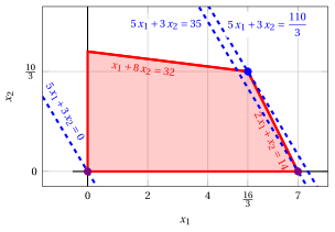
An optimal solution \({ \tilde{\boldsymbol x}}(\, LP\,)\) is:

\[ \tilde{x}_1=\dfrac{16}{3},~~\tilde{x}_2=\dfrac{10}{3} \]

the optimal value \(z(\, LP\,)\) is \(\dfrac{110}{3}.\)

In violet the first and the second vertex explored by the previous execution of the revised simplex algorithm (before reaching the optimal one depicted in blue).

In dashed blue, the contour lines of the objective function associated with the values taken in the three vertices.

Exercise 11.6: Revised simplex algorithm (P5)

Consider the following LP problem in canonical maximization form with \(n=2\) variables and \(m=2\) constraints:

\[ \begin{array}{rrrrrr} {\max} & {2}\, {x_1} & {+} & {3}\, {x_2} \\[2ex] \text{subject to} & {6}\, {x_1} & {+} & {21}\, {x_2} & {\le} & {77} \\[2ex] & {8}\, {x_1} & {+} & {3}\, {x_2} & {\le} & {36} \\[2ex] & {x_1,} & & {x_2} & {\ge} & {0} \end{array} \]

By introducing the slack variables, we get the following LP problem in standard maximization form with \(n+m=4\) variables and \(m=2\) constraints:

\[ \begin{array}{rrrrrrrrrr} {\max} & {2}\, {x_1} & {+} & {3}\, {x_2} \\[2ex] \text{subject to} & {6}\, {x_1} & {+} & {21}\, {x_2} & {+} & {x_3} & & & {=} & {77} \\[2ex] & {8}\, {x_1} & {+} & {3}\, {x_2} & & & {+} & {x_4} & {=} & {36} \\[2ex] & {x_1,} & & {x_2,} & & {x_3,} & & {x_4} & {\ge} & {0} \end{array} \]

Questions

• Execute the revised simplex algorithm to find an optimal solution of this LP problem using Bland's rule to select the pivot column and the pivot row.

Solution

We have:

\[ {\boldsymbol A}= \begin{pmatrix} 6 & 21 & 1 & 0\\ 8 & 3 & 0 & 1 \end{pmatrix} \quad {\boldsymbol b}= \begin{pmatrix} 77\\ 36 \end{pmatrix} \quad {\boldsymbol c}= \begin{pmatrix} 2\\ 3\\ 0\\ 0 \end{pmatrix} \quad {\boldsymbol x}= \begin{pmatrix} x_1 \\ x_2 \\ x_3 \\ x_4 \end{pmatrix} \]

• Initialization

  Since it is an LP problem in standard form obtained from an LP problem in canonical form with \(~{\boldsymbol b} \ge 0\) by adding the slack variables, the partition \(\pazocal{B}=\{3,4\}\) and \(\pazocal{N}=\{1,2\}\) is associated with the following basic feasible solution:

  \[ \begin{pmatrix} x_3 \\ x_4 \end{pmatrix} = \begin{pmatrix} 77\\ 36 \end{pmatrix} \text{ and } \begin{pmatrix} x_1 \\ x_2 \end{pmatrix} = \begin{pmatrix} 0\\ 0 \end{pmatrix} \]

• Iteration 1

  With \(\pazocal{B}= \{3,~~4\}\) and \(\pazocal{N}= \{1,~~2\}\), we have:

  \[ {\boldsymbol x}_{\pazocal{B}}= \begin{pmatrix} x_3 \\ x_4 \end{pmatrix} ~~ {\boldsymbol A}_{\pazocal{B}}= \begin{pmatrix} 1 & 0\\ 0 & 1 \end{pmatrix} ~~ {\boldsymbol c}_{\pazocal{B}}= \begin{pmatrix} 0\\ 0 \end{pmatrix} ~~ {{ \bar{\boldsymbol b}}}= \begin{pmatrix} 77\\ 36 \end{pmatrix} \]
  \[ {\boldsymbol x}_{\pazocal{N}}= \begin{pmatrix} x_1 \\ x_2 \end{pmatrix} ~~ {\boldsymbol A}_{\pazocal{N}}= \begin{pmatrix} 6 & 21\\ 8 & 3 \end{pmatrix} ~~ {\boldsymbol c}_{\pazocal{N}}= \begin{pmatrix} 2\\ 3 \end{pmatrix} \]

  Optimality check

  We solve \({\boldsymbol \pi} \; {\boldsymbol A}_{\pazocal{B}} = {\boldsymbol c}'_{\pazocal{B}}\) to compute \({\boldsymbol \pi} = {{{\boldsymbol c}'_{\pazocal{B}} \; {\boldsymbol A}_{\pazocal{B}}^{-1}}}\), first system of linear equations:

  \[\begin{equation*} \begin{cases} \begin{array}{rrrrr} {\pi_3} & & & {=} & {0} \\[2ex] & & {\pi_4} & {=} & {0} \end{array} \end{cases} \qquad {\boldsymbol \pi}= \begin{pmatrix} 0 & 0\\ \end{pmatrix} \end{equation*}\]

  We compute the basic feasible solution value \({\bar{z}} = {\boldsymbol \pi} \; {\boldsymbol b} = \begin{pmatrix} 0 & 0\\ \end{pmatrix} \begin{pmatrix} 77\\ 36 \end{pmatrix} = 0\)

  We compute the reduced costs \({{ \bar{\boldsymbol c}}'} = {{\boldsymbol c}'_{\pazocal{N}} - {\boldsymbol \pi} \; {\boldsymbol A}_{\pazocal{N}}}\):

  \[ {{ \bar{\boldsymbol c}}'} = \begin{pmatrix} 2 & 3\\ \end{pmatrix} - \begin{pmatrix} 0 & 0\\ \end{pmatrix} \begin{pmatrix} 6 & 21\\ 8 & 3 \end{pmatrix} = \underbrace{ \begin{pmatrix} 2 & 3\\ \end{pmatrix} }_{{c_{1}~~~c_{2}}} - \underbrace{ \begin{pmatrix} 0 & 0\\ \end{pmatrix} }_{{\boldsymbol \pi}\;{\boldsymbol A}_{1} ~~{\boldsymbol \pi}\;{\boldsymbol A}_{2}} = \underbrace{ \begin{pmatrix} 2 & 3\\ \end{pmatrix} }_{{\bar{c}_{1}~~~\bar{c}_{2}}} \]

  Not all reduced costs are non-positive then we perform a pivoting operation.

  Pivoting operation

  Since \({c}_{1} > {\boldsymbol \pi} \;{\boldsymbol A}_{1}\), \(x_1\) is the pivot column and we have \({\boldsymbol A}_{1} = \begin{pmatrix} 6\\ 8 \end{pmatrix}\)

  We solve \({\boldsymbol A}_{\pazocal{B}} \; {\boldsymbol d} = {\boldsymbol A}_{1}\) to compute \({\boldsymbol d}={ {\boldsymbol A}_{\pazocal{B}}^{-1}} {\boldsymbol A}_{1}\), second system of linear equations:

  \[\begin{equation*} \begin{cases} \begin{array}{rrrrr} {d_3} & & & {=} & {6} \\[2ex] & & {d_4} & {=} & {8} \end{array} \end{cases} \qquad {\boldsymbol d}= \begin{pmatrix} 6\\ 8 \end{pmatrix} \end{equation*}\]

  We have to find the largest \(t\) such that \({{ \bar{\boldsymbol b}}} - t \; {{\boldsymbol d}} \ge 0\):

  \[ \begin{cases} \underbrace{77 -t \cdot 6\ge 0}_{x_3 \ge 0} \\[2ex] \underbrace{36 -t \cdot 8\ge 0}_{x_4 \ge 0} \end{cases} \qquad \begin{cases} t\le \dfrac{77}{6} \\[2ex] t\le \dfrac{9}{2} \end{cases} \text{ then } t_{m}=\dfrac{9}{2} \]

  Accordingly the value of the pivot column becomes \(t_{m}\), i.e., \(x_1=\dfrac{9}{2}\). The value of \(x_4\) becomes zero and \(x_4\) is the pivot row. The other basic variables take values \({ \bar{\boldsymbol b}} - t_{m} \; {\boldsymbol d}\), then we have:

  \[ x_3 = 77 - \dfrac{9}{2} \cdot 6 = 50 \]

• Iteration 2

  With \(\pazocal{B}= \{1,~~3\}\) and \(\pazocal{N}= \{2,~~4\}\), we have:

  \[ {\boldsymbol x}_{\pazocal{B}}= \begin{pmatrix} x_1 \\ x_3 \end{pmatrix} ~~ {\boldsymbol A}_{\pazocal{B}}= \begin{pmatrix} 6 & 1\\ 8 & 0 \end{pmatrix} ~~ {\boldsymbol c}_{\pazocal{B}}= \begin{pmatrix} 2\\ 0 \end{pmatrix} ~~ {{ \bar{\boldsymbol b}}}= \begin{pmatrix} \dfrac{9}{2}\\[2ex] 50 \end{pmatrix} \]
  \[ {\boldsymbol x}_{\pazocal{N}}= \begin{pmatrix} x_2 \\ x_4 \end{pmatrix} ~~ {\boldsymbol A}_{\pazocal{N}}= \begin{pmatrix} 21 & 0\\ 3 & 1 \end{pmatrix} ~~ {\boldsymbol c}_{\pazocal{N}}= \begin{pmatrix} 3\\ 0 \end{pmatrix} \]

  Optimality check

  We solve \({\boldsymbol \pi} \; {\boldsymbol A}_{\pazocal{B}} = {\boldsymbol c}'_{\pazocal{B}}\) to compute \({\boldsymbol \pi} = {{{\boldsymbol c}'_{\pazocal{B}} \; {\boldsymbol A}_{\pazocal{B}}^{-1}}}\), first system of linear equations:

  \[\begin{equation*} \begin{cases} \begin{array}{rrrrr} {6}\, {\pi_1} & {+} & {8}\, {\pi_3} & {=} & {2} \\[2ex] {\pi_1} & & & {=} & {0} \end{array} \end{cases} \qquad {\boldsymbol \pi}= \begin{pmatrix} 0 & \dfrac{1}{4}\\ \end{pmatrix} \end{equation*}\]

  We compute the basic feasible solution value \({\bar{z}} = {\boldsymbol \pi} \; {\boldsymbol b} = \begin{pmatrix} 0 & \dfrac{1}{4}\\ \end{pmatrix} \begin{pmatrix} 77\\ 36 \end{pmatrix} = 9\)

  We compute the reduced costs \({{ \bar{\boldsymbol c}}'} = {{\boldsymbol c}'_{\pazocal{N}} - {\boldsymbol \pi} \; {\boldsymbol A}_{\pazocal{N}}}\):

  \[ {{ \bar{\boldsymbol c}}'} = \begin{pmatrix} 3 & 0\\ \end{pmatrix} - \begin{pmatrix} 0 & \dfrac{1}{4}\\ \end{pmatrix} \begin{pmatrix} 21 & 0\\ 3 & 1 \end{pmatrix} = \underbrace{ \begin{pmatrix} 3 & 0\\ \end{pmatrix} }_{{c_{2}~~~c_{4}}} - \underbrace{ \begin{pmatrix} \dfrac{3}{4} & \dfrac{1}{4}\\ \end{pmatrix} }_{{\boldsymbol \pi}\;{\boldsymbol A}_{2} ~~{\boldsymbol \pi}\;{\boldsymbol A}_{4}} = \underbrace{ \begin{pmatrix} \dfrac{9}{4} & -\dfrac{1}{4}\\ \end{pmatrix} }_{{\bar{c}_{2}~~~\bar{c}_{4}}} \]

  Not all reduced costs are non-positive then we perform a pivoting operation.

  Pivoting operation

  Since \({c}_{2} > {\boldsymbol \pi} \;{\boldsymbol A}_{2}\), \(x_2\) is the pivot column and we have \({\boldsymbol A}_{2} = \begin{pmatrix} 21\\ 3 \end{pmatrix}\)

  We solve \({\boldsymbol A}_{\pazocal{B}} \; {\boldsymbol d} = {\boldsymbol A}_{2}\) to compute \({\boldsymbol d}={ {\boldsymbol A}_{\pazocal{B}}^{-1}} {\boldsymbol A}_{2}\), second system of linear equations:

  \[\begin{equation*} \begin{cases} \begin{array}{rrrrr} {6}\, {d_1} & {+} & {d_3} & {=} & {21} \\[2ex] {8}\, {d_1} & & & {=} & {3} \end{array} \end{cases} \qquad {\boldsymbol d}= \begin{pmatrix} \dfrac{3}{8}\\[2ex] \dfrac{75}{4} \end{pmatrix} \end{equation*}\]

  We have to find the largest \(t\) such that \({{ \bar{\boldsymbol b}}} - t \; {{\boldsymbol d}} \ge 0\):

  \[ \begin{cases} \underbrace{\dfrac{9}{2} -t \cdot \dfrac{3}{8}\ge 0}_{x_1 \ge 0} \\[2ex] \underbrace{50 -t \cdot \dfrac{75}{4}\ge 0}_{x_3 \ge 0} \end{cases} \qquad \begin{cases} t\le 12 \\[2ex] t\le \dfrac{8}{3} \end{cases} \text{ then } t_{m}=\dfrac{8}{3} \]

  Accordingly the value of the pivot column becomes \(t_{m}\), i.e., \(x_2=\dfrac{8}{3}\). The value of \(x_3\) becomes zero and \(x_3\) is the pivot row. The other basic variables take values \({ \bar{\boldsymbol b}} - t_{m} \; {\boldsymbol d}\), then we have:

  \[ x_1 = \dfrac{9}{2} - \dfrac{8}{3} \cdot \dfrac{3}{8} = \dfrac{7}{2} \]

• Iteration 3

  With \(\pazocal{B}= \{1,~~2\}\) and \(\pazocal{N}= \{3,~~4\}\), we have:

  \[ {\boldsymbol x}_{\pazocal{B}}= \begin{pmatrix} x_1 \\ x_2 \end{pmatrix} ~~ {\boldsymbol A}_{\pazocal{B}}= \begin{pmatrix} 6 & 21\\ 8 & 3 \end{pmatrix} ~~ {\boldsymbol c}_{\pazocal{B}}= \begin{pmatrix} 2\\ 3 \end{pmatrix} ~~ {{ \bar{\boldsymbol b}}}= \begin{pmatrix} \dfrac{7}{2}\\[2ex] \dfrac{8}{3} \end{pmatrix} \]
  \[ {\boldsymbol x}_{\pazocal{N}}= \begin{pmatrix} x_3 \\ x_4 \end{pmatrix} ~~ {\boldsymbol A}_{\pazocal{N}}= \begin{pmatrix} 1 & 0\\ 0 & 1 \end{pmatrix} ~~ {\boldsymbol c}_{\pazocal{N}}= \begin{pmatrix} 0\\ 0 \end{pmatrix} \]

  Optimality check

  We solve \({\boldsymbol \pi} \; {\boldsymbol A}_{\pazocal{B}} = {\boldsymbol c}'_{\pazocal{B}}\) to compute \({\boldsymbol \pi} = {{{\boldsymbol c}'_{\pazocal{B}} \; {\boldsymbol A}_{\pazocal{B}}^{-1}}}\), first system of linear equations:

  \[\begin{equation*} \begin{cases} \begin{array}{rrrrr} {6}\, {\pi_1} & {+} & {8}\, {\pi_2} & {=} & {2} \\[2ex] {21}\, {\pi_1} & {+} & {3}\, {\pi_2} & {=} & {3} \end{array} \end{cases} \qquad {\boldsymbol \pi}= \begin{pmatrix} \dfrac{3}{25} & \dfrac{4}{25}\\ \end{pmatrix} \end{equation*}\]

  We compute the basic feasible solution value \({\bar{z}} = {\boldsymbol \pi} \; {\boldsymbol b} = \begin{pmatrix} \dfrac{3}{25} & \dfrac{4}{25}\\ \end{pmatrix} \begin{pmatrix} 77\\ 36 \end{pmatrix} = 15\)

  We compute the reduced costs \({{ \bar{\boldsymbol c}}'} = {{\boldsymbol c}'_{\pazocal{N}} - {\boldsymbol \pi} \; {\boldsymbol A}_{\pazocal{N}}}\):

  \[ {{ \bar{\boldsymbol c}}'} = \begin{pmatrix} 0 & 0\\ \end{pmatrix} - \begin{pmatrix} \dfrac{3}{25} & \dfrac{4}{25}\\ \end{pmatrix} \begin{pmatrix} 1 & 0\\ 0 & 1 \end{pmatrix} = \underbrace{ \begin{pmatrix} 0 & 0\\ \end{pmatrix} }_{{c_{3}~~~c_{4}}} - \underbrace{ \begin{pmatrix} \dfrac{3}{25} & \dfrac{4}{25}\\ \end{pmatrix} }_{{\boldsymbol \pi}\;{\boldsymbol A}_{3} ~~{\boldsymbol \pi}\;{\boldsymbol A}_{4}} = \underbrace{ \begin{pmatrix} -\dfrac{3}{25} & -\dfrac{4}{25}\\ \end{pmatrix} }_{{\bar{c}_{3}~~~\bar{c}_{4}}} \]

  All reduced costs are non-positive, then the basic feasible solution

  \[ {\boldsymbol x}_{\pazocal{B}}= \begin{pmatrix} x_1 \\ x_2 \end{pmatrix}=\begin{pmatrix} \dfrac{7}{2}\\[2ex] \dfrac{8}{3} \end{pmatrix} \text{ and } {\boldsymbol x}_{\pazocal{N}}= \begin{pmatrix} x_3 \\ x_4 \end{pmatrix}=\begin{pmatrix} 0\\ 0 \end{pmatrix} \]

  is an optimal solution of the LP problem and \({\bar{z}} = 15\) is the optimal solution value.

Graphical solution:

The feasible region of the LP problem (in canonical form) is the polyhedron shaded in red:

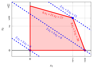
An optimal solution \({ \tilde{\boldsymbol x}}(\,LP\,)\) is:

\[ \tilde{x}_1=\dfrac{7}{2},~~\tilde{x}_2=\dfrac{8}{3} \]

the optimal value \(z(\, LP\,)\) is \(15.\)

In violet the first and the second vertex explored by the previous execution of the revised simplex algorithm (before reaching the optimal one depicted in blue).

In dashed blue, the contour lines of the objective function associated with the values taken in the three vertices.

Exercise 11.7: Revised simplex algorithm (P6)

Consider the following LP problem in canonical maximization form with \(n=2\) variables and \(m=2\) constraints:

\[ \begin{array}{rrrrrr} {\max} & {x_1} & {+} & {x_2} \\[2ex] \text{subject to} & {4}\, {x_1} & {+} & {15}\, {x_2} & {\le} & {70} \\[2ex] & {12}\, {x_1} & {+} & {3}\, {x_2} & {\le} & {52} \\[2ex] & {x_1,} & & {x_2} & {\ge} & {0} \end{array} \]

By introducing the slack variables, we get the following LP problem in standard maximization form with \(n+m=4\) variables and \(m=2\) constraints:

\[ \begin{array}{rrrrrrrrrr} {\max} & {x_1} & {+} & {x_2} \\[2ex] \text{subject to} & {4}\, {x_1} & {+} & {15}\, {x_2} & {+} & {x_3} & & & {=} & {70} \\[2ex] & {12}\, {x_1} & {+} & {3}\, {x_2} & & & {+} & {x_4} & {=} & {52} \\[2ex] & {x_1,} & & {x_2,} & & {x_3,} & & {x_4} & {\ge} & {0} \end{array} \]

Questions

• Execute the revised simplex algorithm to find an optimal solution of this LP problem using Bland's rule to select the pivot column and the pivot row.

Solution

We have:

\[ {\boldsymbol A}= \begin{pmatrix} 4 & 15 & 1 & 0\\ 12 & 3 & 0 & 1 \end{pmatrix} \quad {\boldsymbol b}= \begin{pmatrix} 70\\ 52 \end{pmatrix} \quad {\boldsymbol c}= \begin{pmatrix} 1\\ 1\\ 0\\ 0 \end{pmatrix} \quad {\boldsymbol x}= \begin{pmatrix} x_1 \\ x_2 \\ x_3 \\ x_4 \end{pmatrix} \]

• Initialization

  Since it is an LP problem in standard form obtained from an LP problem in canonical form with \(~{\boldsymbol b} \ge 0\) by adding the slack variables, the partition \(\pazocal{B}=\{3,4\}\) and \(\pazocal{N}=\{1,2\}\) is associated with the following basic feasible solution:

  \[ \begin{pmatrix} x_3 \\ x_4 \end{pmatrix} = \begin{pmatrix} 70\\ 52 \end{pmatrix} \text{ and } \begin{pmatrix} x_1 \\ x_2 \end{pmatrix} = \begin{pmatrix} 0\\ 0 \end{pmatrix} \]

• Iteration 1

  With \(\pazocal{B}= \{3,~~4\}\) and \(\pazocal{N}= \{1,~~2\}\), we have:

  \[ {\boldsymbol x}_{\pazocal{B}}= \begin{pmatrix} x_3 \\ x_4 \end{pmatrix} ~~ {\boldsymbol A}_{\pazocal{B}}= \begin{pmatrix} 1 & 0\\ 0 & 1 \end{pmatrix} ~~ {\boldsymbol c}_{\pazocal{B}}= \begin{pmatrix} 0\\ 0 \end{pmatrix} ~~ {{ \bar{\boldsymbol b}}}= \begin{pmatrix} 70\\ 52 \end{pmatrix} \]
  \[ {\boldsymbol x}_{\pazocal{N}}= \begin{pmatrix} x_1 \\ x_2 \end{pmatrix} ~~ {\boldsymbol A}_{\pazocal{N}}= \begin{pmatrix} 4 & 15\\ 12 & 3 \end{pmatrix} ~~ {\boldsymbol c}_{\pazocal{N}}= \begin{pmatrix} 1\\ 1 \end{pmatrix} \]

  Optimality check

  We solve \({\boldsymbol \pi} \; {\boldsymbol A}_{\pazocal{B}} = {\boldsymbol c}'_{\pazocal{B}}\) to compute \({\boldsymbol \pi} = {{{\boldsymbol c}'_{\pazocal{B}} \; {\boldsymbol A}_{\pazocal{B}}^{-1}}}\), first system of linear equations:

  \[\begin{equation*} \begin{cases} \begin{array}{rrrrr} {\pi_3} & & & {=} & {0} \\[2ex] & & {\pi_4} & {=} & {0} \end{array} \end{cases} \qquad {\boldsymbol \pi}= \begin{pmatrix} 0 & 0\\ \end{pmatrix} \end{equation*}\]

  We compute the basic feasible solution value \({\bar{z}} = {\boldsymbol \pi} \; {\boldsymbol b} = \begin{pmatrix} 0 & 0\\ \end{pmatrix} \begin{pmatrix} 70\\ 52 \end{pmatrix} = 0\)

  We compute the reduced costs \({{ \bar{\boldsymbol c}}'} = {{\boldsymbol c}'_{\pazocal{N}} - {\boldsymbol \pi} \; {\boldsymbol A}_{\pazocal{N}}}\):

  \[ {{ \bar{\boldsymbol c}}'} = \begin{pmatrix} 1 & 1\\ \end{pmatrix} - \begin{pmatrix} 0 & 0\\ \end{pmatrix} \begin{pmatrix} 4 & 15\\ 12 & 3 \end{pmatrix} = \underbrace{ \begin{pmatrix} 1 & 1\\ \end{pmatrix} }_{{c_{1}~~~c_{2}}} - \underbrace{ \begin{pmatrix} 0 & 0\\ \end{pmatrix} }_{{\boldsymbol \pi}\;{\boldsymbol A}_{1} ~~{\boldsymbol \pi}\;{\boldsymbol A}_{2}} = \underbrace{ \begin{pmatrix} 1 & 1\\ \end{pmatrix} }_{{\bar{c}_{1}~~~\bar{c}_{2}}} \]

  Not all reduced costs are non-positive then we perform a pivoting operation.

  Pivoting operation

  Since \({c}_{1} > {\boldsymbol \pi} \;{\boldsymbol A}_{1}\), \(x_1\) is the pivot column and we have \({\boldsymbol A}_{1} = \begin{pmatrix} 4\\ 12 \end{pmatrix}\)

  We solve \({\boldsymbol A}_{\pazocal{B}} \; {\boldsymbol d} = {\boldsymbol A}_{1}\) to compute \({\boldsymbol d}={ {\boldsymbol A}_{\pazocal{B}}^{-1}} {\boldsymbol A}_{1}\), second system of linear equations:

  \[\begin{equation*} \begin{cases} \begin{array}{rrrrr} {d_3} & & & {=} & {4} \\[2ex] & & {d_4} & {=} & {12} \end{array} \end{cases} \qquad {\boldsymbol d}= \begin{pmatrix} 4\\ 12 \end{pmatrix} \end{equation*}\]

  We have to find the largest \(t\) such that \({{ \bar{\boldsymbol b}}} - t \; {{\boldsymbol d}} \ge 0\):

  \[ \begin{cases} \underbrace{70 -t \cdot 4\ge 0}_{x_3 \ge 0} \\[2ex] \underbrace{52 -t \cdot 12\ge 0}_{x_4 \ge 0} \end{cases} \qquad \begin{cases} t\le \dfrac{35}{2} \\[2ex] t\le \dfrac{13}{3} \end{cases} \text{ then } t_{m}=\dfrac{13}{3} \]

  Accordingly the value of the pivot column becomes \(t_{m}\), i.e., \(x_1=\dfrac{13}{3}\). The value of \(x_4\) becomes zero and \(x_4\) is the pivot row. The other basic variables take values \({ \bar{\boldsymbol b}} - t_{m} \; {\boldsymbol d}\), then we have:

  \[ x_3 = 70 - \dfrac{13}{3} \cdot 4 = \dfrac{158}{3} \]

• Iteration 2

  With \(\pazocal{B}= \{1,~~3\}\) and \(\pazocal{N}= \{2,~~4\}\), we have:

  \[ {\boldsymbol x}_{\pazocal{B}}= \begin{pmatrix} x_1 \\ x_3 \end{pmatrix} ~~ {\boldsymbol A}_{\pazocal{B}}= \begin{pmatrix} 4 & 1\\ 12 & 0 \end{pmatrix} ~~ {\boldsymbol c}_{\pazocal{B}}= \begin{pmatrix} 1\\ 0 \end{pmatrix} ~~ {{ \bar{\boldsymbol b}}}= \begin{pmatrix} \dfrac{13}{3}\\[2ex] \dfrac{158}{3} \end{pmatrix} \]
  \[ {\boldsymbol x}_{\pazocal{N}}= \begin{pmatrix} x_2 \\ x_4 \end{pmatrix} ~~ {\boldsymbol A}_{\pazocal{N}}= \begin{pmatrix} 15 & 0\\ 3 & 1 \end{pmatrix} ~~ {\boldsymbol c}_{\pazocal{N}}= \begin{pmatrix} 1\\ 0 \end{pmatrix} \]

  Optimality check

  We solve \({\boldsymbol \pi} \; {\boldsymbol A}_{\pazocal{B}} = {\boldsymbol c}'_{\pazocal{B}}\) to compute \({\boldsymbol \pi} = {{{\boldsymbol c}'_{\pazocal{B}} \; {\boldsymbol A}_{\pazocal{B}}^{-1}}}\), first system of linear equations:

  \[\begin{equation*} \begin{cases} \begin{array}{rrrrr} {4}\, {\pi_1} & {+} & {12}\, {\pi_3} & {=} & {1} \\[2ex] {\pi_1} & & & {=} & {0} \end{array} \end{cases} \qquad {\boldsymbol \pi}= \begin{pmatrix} 0 & \dfrac{1}{12}\\ \end{pmatrix} \end{equation*}\]

  We compute the basic feasible solution value \({\bar{z}} = {\boldsymbol \pi} \; {\boldsymbol b} = \begin{pmatrix} 0 & \dfrac{1}{12}\\ \end{pmatrix} \begin{pmatrix} 70\\ 52 \end{pmatrix} = \dfrac{13}{3}\)

  We compute the reduced costs \({{ \bar{\boldsymbol c}}'} = {{\boldsymbol c}'_{\pazocal{N}} - {\boldsymbol \pi} \; {\boldsymbol A}_{\pazocal{N}}}\):

  \[ {{ \bar{\boldsymbol c}}'} = \begin{pmatrix} 1 & 0\\ \end{pmatrix} - \begin{pmatrix} 0 & \dfrac{1}{12}\\ \end{pmatrix} \begin{pmatrix} 15 & 0\\ 3 & 1 \end{pmatrix} = \underbrace{ \begin{pmatrix} 1 & 0\\ \end{pmatrix} }_{{c_{2}~~~c_{4}}} - \underbrace{ \begin{pmatrix} \dfrac{1}{4} & \dfrac{1}{12}\\ \end{pmatrix} }_{{\boldsymbol \pi}\;{\boldsymbol A}_{2} ~~{\boldsymbol \pi}\;{\boldsymbol A}_{4}} = \underbrace{ \begin{pmatrix} \dfrac{3}{4} & -\dfrac{1}{12}\\ \end{pmatrix} }_{{\bar{c}_{2}~~~\bar{c}_{4}}} \]

  Not all reduced costs are non-positive then we perform a pivoting operation.

  Pivoting operation

  Since \({c}_{2} > {\boldsymbol \pi} \;{\boldsymbol A}_{2}\), \(x_2\) is the pivot column and we have \({\boldsymbol A}_{2} = \begin{pmatrix} 15\\ 3 \end{pmatrix}\)

  We solve \({\boldsymbol A}_{\pazocal{B}} \; {\boldsymbol d} = {\boldsymbol A}_{2}\) to compute \({\boldsymbol d}={ {\boldsymbol A}_{\pazocal{B}}^{-1}} {\boldsymbol A}_{2}\), second system of linear equations:

  \[\begin{equation*} \begin{cases} \begin{array}{rrrrr} {4}\, {d_1} & {+} & {d_3} & {=} & {15} \\[2ex] {12}\, {d_1} & & & {=} & {3} \end{array} \end{cases} \qquad {\boldsymbol d}= \begin{pmatrix} \dfrac{1}{4}\\[2ex] 14 \end{pmatrix} \end{equation*}\]

  We have to find the largest \(t\) such that \({{ \bar{\boldsymbol b}}} - t \; {{\boldsymbol d}} \ge 0\):

  \[ \begin{cases} \underbrace{\dfrac{13}{3} -t \cdot \dfrac{1}{4}\ge 0}_{x_1 \ge 0} \\[2ex] \underbrace{\dfrac{158}{3} -t \cdot 14\ge 0}_{x_3 \ge 0} \end{cases} \qquad \begin{cases} t\le \dfrac{52}{3} \\[2ex] t\le \dfrac{79}{21} \end{cases} \text{ then } t_{m}=\dfrac{79}{21} \]

  Accordingly the value of the pivot column becomes \(t_{m}\), i.e., \(x_2=\dfrac{79}{21}\). The value of \(x_3\) becomes zero and \(x_3\) is the pivot row. The other basic variables take values \({ \bar{\boldsymbol b}} - t_{m} \; {\boldsymbol d}\), then we have:

  \[ x_1 = \dfrac{13}{3} - \dfrac{79}{21} \cdot \dfrac{1}{4} = \dfrac{95}{28} \]

• Iteration 3

  With \(\pazocal{B}= \{1,~~2\}\) and \(\pazocal{N}= \{3,~~4\}\), we have:

  \[ {\boldsymbol x}_{\pazocal{B}}= \begin{pmatrix} x_1 \\ x_2 \end{pmatrix} ~~ {\boldsymbol A}_{\pazocal{B}}= \begin{pmatrix} 4 & 15\\ 12 & 3 \end{pmatrix} ~~ {\boldsymbol c}_{\pazocal{B}}= \begin{pmatrix} 1\\ 1 \end{pmatrix} ~~ {{ \bar{\boldsymbol b}}}= \begin{pmatrix} \dfrac{95}{28}\\[2ex] \dfrac{79}{21} \end{pmatrix} \]
  \[ {\boldsymbol x}_{\pazocal{N}}= \begin{pmatrix} x_3 \\ x_4 \end{pmatrix} ~~ {\boldsymbol A}_{\pazocal{N}}= \begin{pmatrix} 1 & 0\\ 0 & 1 \end{pmatrix} ~~ {\boldsymbol c}_{\pazocal{N}}= \begin{pmatrix} 0\\ 0 \end{pmatrix} \]

  Optimality check

  We solve \({\boldsymbol \pi} \; {\boldsymbol A}_{\pazocal{B}} = {\boldsymbol c}'_{\pazocal{B}}\) to compute \({\boldsymbol \pi} = {{{\boldsymbol c}'_{\pazocal{B}} \; {\boldsymbol A}_{\pazocal{B}}^{-1}}}\), first system of linear equations:

  \[\begin{equation*} \begin{cases} \begin{array}{rrrrr} {4}\, {\pi_1} & {+} & {12}\, {\pi_2} & {=} & {1} \\[2ex] {15}\, {\pi_1} & {+} & {3}\, {\pi_2} & {=} & {1} \end{array} \end{cases} \qquad {\boldsymbol \pi}= \begin{pmatrix} \dfrac{3}{56} & \dfrac{11}{168}\\ \end{pmatrix} \end{equation*}\]

  We compute the basic feasible solution value \({\bar{z}} = {\boldsymbol \pi} \; {\boldsymbol b} = \begin{pmatrix} \dfrac{3}{56} & \dfrac{11}{168}\\ \end{pmatrix} \begin{pmatrix} 70\\ 52 \end{pmatrix} = \dfrac{601}{84}\)

  We compute the reduced costs \({{ \bar{\boldsymbol c}}'} = {{\boldsymbol c}'_{\pazocal{N}} - {\boldsymbol \pi} \; {\boldsymbol A}_{\pazocal{N}}}\):

  \[ {{ \bar{\boldsymbol c}}'} = \begin{pmatrix} 0 & 0\\ \end{pmatrix} - \begin{pmatrix} \dfrac{3}{56} & \dfrac{11}{168}\\ \end{pmatrix} \begin{pmatrix} 1 & 0\\ 0 & 1 \end{pmatrix} = \underbrace{ \begin{pmatrix} 0 & 0\\ \end{pmatrix} }_{{c_{3}~~~c_{4}}} - \underbrace{ \begin{pmatrix} \dfrac{3}{56} & \dfrac{11}{168}\\ \end{pmatrix} }_{{\boldsymbol \pi}\;{\boldsymbol A}_{3} ~~{\boldsymbol \pi}\;{\boldsymbol A}_{4}} = \underbrace{ \begin{pmatrix} -\dfrac{3}{56} & -\dfrac{11}{168}\\ \end{pmatrix} }_{{\bar{c}_{3}~~~\bar{c}_{4}}} \]

  All reduced costs are non-positive, then the basic feasible solution

  \[ {\boldsymbol x}_{\pazocal{B}}= \begin{pmatrix} x_1 \\ x_2 \end{pmatrix}=\begin{pmatrix} \dfrac{95}{28}\\[2ex] \dfrac{79}{21} \end{pmatrix} \text{ and } {\boldsymbol x}_{\pazocal{N}}= \begin{pmatrix} x_3 \\ x_4 \end{pmatrix}=\begin{pmatrix} 0\\ 0 \end{pmatrix} \]

  is an optimal solution of the LP problem and \({\bar{z}} = \dfrac{601}{84}\) is the optimal solution value.

Graphical solution:

The feasible region of the LP problem (in canonical form) is the polyhedron shaded in red:

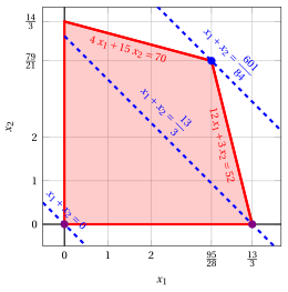
An optimal solution \({ \tilde{\boldsymbol x}}(\,LP\,)\) is:

\[ \tilde{x}_1=\dfrac{95}{28},~~\tilde{x}_2=\dfrac{79}{21} \]

the optimal value \(z(\, LP\,)\) is \(\dfrac{601}{84}.\)

In violet the first and the second vertex explored by the previous execution of the revised simplex algorithm (before reaching the optimal one depicted in blue).

In dashed blue, the contour lines of the objective function associated with the values taken in the three vertices.

Exercise 11.8: Revised simplex algorithm (P7)

Consider the following LP problem in canonical maximization form with \(n=2\) variables and \(m=2\) constraints:

\[ \begin{array}{rrrrrr} {\max} & {3}\, {x_1} & {+} & {x_2} \\[2ex] \text{subject to} & {x_1} & {+} & {4}\, {x_2} & {\le} & {12} \\[2ex] & {2}\, {x_1} & {+} & {x_2} & {\le} & {5} \\[2ex] & {x_1,} & & {x_2} & {\ge} & {0} \end{array} \]

By introducing the slack variables, we get the following LP problem in standard maximization form with \(n+m=4\) variables and \(m=2\) constraints:

\[ \begin{array}{rrrrrrrrrr} {\max} & {3}\, {x_1} & {+} & {x_2} \\[2ex] \text{subject to} & {x_1} & {+} & {4}\, {x_2} & {+} & {x_3} & & & {=} & {12} \\[2ex] & {2}\, {x_1} & {+} & {x_2} & & & {+} & {x_4} & {=} & {5} \\[2ex] & {x_1,} & & {x_2,} & & {x_3,} & & {x_4} & {\ge} & {0} \end{array} \]

Questions

• Execute the revised simplex algorithm to find an optimal solution of this LP problem using Bland's rule to select the pivot column and the pivot row.

Solution

We have:

\[ {\boldsymbol A}= \begin{pmatrix} 1 & 4 & 1 & 0\\ 2 & 1 & 0 & 1 \end{pmatrix} \quad {\boldsymbol b}= \begin{pmatrix} 12\\ 5 \end{pmatrix} \quad {\boldsymbol c}= \begin{pmatrix} 3\\ 1\\ 0\\ 0 \end{pmatrix} \quad {\boldsymbol x}= \begin{pmatrix} x_1 \\ x_2 \\ x_3 \\ x_4 \end{pmatrix} \]

• Initialization

  Since it is an LP problem in standard form obtained from an LP problem in canonical form with \(~{\boldsymbol b} \ge 0\) by adding the slack variables, the partition \(\pazocal{B}=\{3,4\}\) and \(\pazocal{N}=\{1,2\}\) is associated with the following basic feasible solution:

  \[ \begin{pmatrix} x_3 \\ x_4 \end{pmatrix} = \begin{pmatrix} 12\\ 5 \end{pmatrix} \text{ and } \begin{pmatrix} x_1 \\ x_2 \end{pmatrix} = \begin{pmatrix} 0\\ 0 \end{pmatrix} \]

• Iteration 1

  With \(\pazocal{B}= \{3,~~4\}\) and \(\pazocal{N}= \{1,~~2\}\), we have:

  \[ {\boldsymbol x}_{\pazocal{B}}= \begin{pmatrix} x_3 \\ x_4 \end{pmatrix} ~~ {\boldsymbol A}_{\pazocal{B}}= \begin{pmatrix} 1 & 0\\ 0 & 1 \end{pmatrix} ~~ {\boldsymbol c}_{\pazocal{B}}= \begin{pmatrix} 0\\ 0 \end{pmatrix} ~~ {{ \bar{\boldsymbol b}}}= \begin{pmatrix} 12\\ 5 \end{pmatrix} \]
  \[ {\boldsymbol x}_{\pazocal{N}}= \begin{pmatrix} x_1 \\ x_2 \end{pmatrix} ~~ {\boldsymbol A}_{\pazocal{N}}= \begin{pmatrix} 1 & 4\\ 2 & 1 \end{pmatrix} ~~ {\boldsymbol c}_{\pazocal{N}}= \begin{pmatrix} 3\\ 1 \end{pmatrix} \]

  Optimality check

  We solve \({\boldsymbol \pi} \; {\boldsymbol A}_{\pazocal{B}} = {\boldsymbol c}'_{\pazocal{B}}\) to compute \({\boldsymbol \pi} = {{{\boldsymbol c}'_{\pazocal{B}} \; {\boldsymbol A}_{\pazocal{B}}^{-1}}}\), first system of linear equations:

  \[\begin{equation*} \begin{cases} \begin{array}{rrrrr} {\pi_3} & & & {=} & {0} \\[2ex] & & {\pi_4} & {=} & {0} \end{array} \end{cases} \qquad {\boldsymbol \pi}= \begin{pmatrix} 0 & 0\\ \end{pmatrix} \end{equation*}\]

  We compute the basic feasible solution value \({\bar{z}} = {\boldsymbol \pi} \; {\boldsymbol b} = \begin{pmatrix} 0 & 0\\ \end{pmatrix} \begin{pmatrix} 12\\ 5 \end{pmatrix} = 0\)

  We compute the reduced costs \({{ \bar{\boldsymbol c}}'} = {{\boldsymbol c}'_{\pazocal{N}} - {\boldsymbol \pi} \; {\boldsymbol A}_{\pazocal{N}}}\):

  \[ {{ \bar{\boldsymbol c}}'} = \begin{pmatrix} 3 & 1\\ \end{pmatrix} - \begin{pmatrix} 0 & 0\\ \end{pmatrix} \begin{pmatrix} 1 & 4\\ 2 & 1 \end{pmatrix} = \underbrace{ \begin{pmatrix} 3 & 1\\ \end{pmatrix} }_{{c_{1}~~~c_{2}}} - \underbrace{ \begin{pmatrix} 0 & 0\\ \end{pmatrix} }_{{\boldsymbol \pi}\;{\boldsymbol A}_{1} ~~{\boldsymbol \pi}\;{\boldsymbol A}_{2}} = \underbrace{ \begin{pmatrix} 3 & 1\\ \end{pmatrix} }_{{\bar{c}_{1}~~~\bar{c}_{2}}} \]

  Not all reduced costs are non-positive then we perform a pivoting operation.

  Pivoting operation

  Since \({c}_{1} > {\boldsymbol \pi} \;{\boldsymbol A}_{1}\), \(x_1\) is the pivot column and we have \({\boldsymbol A}_{1} = \begin{pmatrix} 1\\ 2 \end{pmatrix}\)

  We solve \({\boldsymbol A}_{\pazocal{B}} \; {\boldsymbol d} = {\boldsymbol A}_{1}\) to compute \({\boldsymbol d}={ {\boldsymbol A}_{\pazocal{B}}^{-1}} {\boldsymbol A}_{1}\), second system of linear equations:

  \[\begin{equation*} \begin{cases} \begin{array}{rrrrr} {d_3} & & & {=} & {1} \\[2ex] & & {d_4} & {=} & {2} \end{array} \end{cases} \qquad {\boldsymbol d}= \begin{pmatrix} 1\\ 2 \end{pmatrix} \end{equation*}\]

  We have to find the largest \(t\) such that \({{ \bar{\boldsymbol b}}} - t \; {{\boldsymbol d}} \ge 0\):

  \[ \begin{cases} \underbrace{12 -t \cdot 1\ge 0}_{x_3 \ge 0} \\[2ex] \underbrace{5 -t \cdot 2\ge 0}_{x_4 \ge 0} \end{cases} \qquad \begin{cases} t\le 12 \\[2ex] t\le \dfrac{5}{2} \end{cases} \text{ then } t_{m}=\dfrac{5}{2} \]

  Accordingly the value of the pivot column becomes \(t_{m}\), i.e., \(x_1=\dfrac{5}{2}\). The value of \(x_4\) becomes zero and \(x_4\) is the pivot row. The other basic variables take values \({ \bar{\boldsymbol b}} - t_{m} \; {\boldsymbol d}\), then we have:

  \[ x_3 = 12 - \dfrac{5}{2} \cdot 1 = \dfrac{19}{2} \]

• Iteration 2

  With \(\pazocal{B}= \{1,~~3\}\) and \(\pazocal{N}= \{2,~~4\}\), we have:

  \[ {\boldsymbol x}_{\pazocal{B}}= \begin{pmatrix} x_1 \\ x_3 \end{pmatrix} ~~ {\boldsymbol A}_{\pazocal{B}}= \begin{pmatrix} 1 & 1\\ 2 & 0 \end{pmatrix} ~~ {\boldsymbol c}_{\pazocal{B}}= \begin{pmatrix} 3\\ 0 \end{pmatrix} ~~ {{ \bar{\boldsymbol b}}}= \begin{pmatrix} \dfrac{5}{2}\\[2ex] \dfrac{19}{2} \end{pmatrix} \]
  \[ {\boldsymbol x}_{\pazocal{N}}= \begin{pmatrix} x_2 \\ x_4 \end{pmatrix} ~~ {\boldsymbol A}_{\pazocal{N}}= \begin{pmatrix} 4 & 0\\ 1 & 1 \end{pmatrix} ~~ {\boldsymbol c}_{\pazocal{N}}= \begin{pmatrix} 1\\ 0 \end{pmatrix} \]

  Optimality check

  We solve \({\boldsymbol \pi} \; {\boldsymbol A}_{\pazocal{B}} = {\boldsymbol c}'_{\pazocal{B}}\) to compute \({\boldsymbol \pi} = {{{\boldsymbol c}'_{\pazocal{B}} \; {\boldsymbol A}_{\pazocal{B}}^{-1}}}\), first system of linear equations:

  \[\begin{equation*} \begin{cases} \begin{array}{rrrrr} {\pi_1} & {+} & {2}\, {\pi_3} & {=} & {3} \\[2ex] {\pi_1} & & & {=} & {0} \end{array} \end{cases} \qquad {\boldsymbol \pi}= \begin{pmatrix} 0 & \dfrac{3}{2}\\ \end{pmatrix} \end{equation*}\]

  We compute the basic feasible solution value \({\bar{z}} = {\boldsymbol \pi} \; {\boldsymbol b} = \begin{pmatrix} 0 & \dfrac{3}{2}\\ \end{pmatrix} \begin{pmatrix} 12\\ 5 \end{pmatrix} = \dfrac{15}{2}\)

  We compute the reduced costs \({{ \bar{\boldsymbol c}}'} = {{\boldsymbol c}'_{\pazocal{N}} - {\boldsymbol \pi} \; {\boldsymbol A}_{\pazocal{N}}}\):

  \[ {{ \bar{\boldsymbol c}}'} = \begin{pmatrix} 1 & 0\\ \end{pmatrix} - \begin{pmatrix} 0 & \dfrac{3}{2}\\ \end{pmatrix} \begin{pmatrix} 4 & 0\\ 1 & 1 \end{pmatrix} = \underbrace{ \begin{pmatrix} 1 & 0\\ \end{pmatrix} }_{{c_{2}~~~c_{4}}} - \underbrace{ \begin{pmatrix} \dfrac{3}{2} & \dfrac{3}{2}\\ \end{pmatrix} }_{{\boldsymbol \pi}\;{\boldsymbol A}_{2} ~~{\boldsymbol \pi}\;{\boldsymbol A}_{4}} = \underbrace{ \begin{pmatrix} -\dfrac{1}{2} & -\dfrac{3}{2}\\ \end{pmatrix} }_{{\bar{c}_{2}~~~\bar{c}_{4}}} \]

  All reduced costs are non-positive, then the basic feasible solution

  \[ {\boldsymbol x}_{\pazocal{B}}= \begin{pmatrix} x_1 \\ x_3 \end{pmatrix}=\begin{pmatrix} \dfrac{5}{2}\\[2ex] \dfrac{19}{2} \end{pmatrix} \text{ and } {\boldsymbol x}_{\pazocal{N}}= \begin{pmatrix} x_2 \\ x_4 \end{pmatrix}=\begin{pmatrix} 0\\ 0 \end{pmatrix} \]

  is an optimal solution of the LP problem and \({\bar{z}} = \dfrac{15}{2}\) is the optimal solution value.

Graphical solution:

The feasible region of the LP problem (in canonical form) is the polyhedron shaded in red:

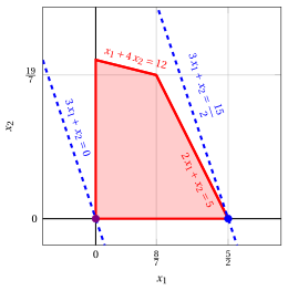
An optimal solution \({ \tilde{\boldsymbol x}}(\, LP\,)\) is:

\[ \tilde{x}_1=\dfrac{5}{2},~~\tilde{x}_2=0 \]

the optimal value \(z(\, LP\,)\) is \(\dfrac{15}{2}.\)

In violet the first vertex explored by the previous execution of the revised simplex algorithm (before reaching the optimal one depicted in blue).

In dashed blue, the contour lines of the objective function associated with the values taken in the two vertices.

Exercise 11.9: Revised simplex algorithm (P8)

Consider the following LP problem in canonical maximization form with \(n=2\) variables and \(m=2\) constraints:

\[ \begin{array}{rrrrrr} {\max} & {x_1} & {+} & {2}\, {x_2} \\[2ex] \text{subject to} & {-x_1} & {+} & {2}\, {x_2} & {\le} & {2} \\[2ex] & {x_1} & {+} & {x_2} & {\le} & {3} \\[2ex] & {x_1,} & & {x_2} & {\ge} & {0} \end{array} \]

By introducing the slack variables, we get the following LP problem in standard maximization form with \(n+m=4\) variables and \(m=2\) constraints:

\[ \begin{array}{rrrrrrrrrr} {\max} & {x_1} & {+} & {2}\, {x_2} \\[2ex] \text{subject to} & {-x_1} & {+} & {2}\, {x_2} & {+} & {x_3} & & & {=} & {2} \\[2ex] & {x_1} & {+} & {x_2} & & & {+} & {x_4} & {=} & {3} \\[2ex] & {x_1,} & & {x_2,} & & {x_3,} & & {x_4} & {\ge} & {0} \end{array} \]

Questions

• Execute the revised simplex algorithm to find an optimal solution of this LP problem using Bland's rule to select the pivot column and the pivot row.

Solution

We have:

\[ {\boldsymbol A}= \begin{pmatrix} -1 & 2 & 1 & 0\\ 1 & 1 & 0 & 1 \end{pmatrix} \quad {\boldsymbol b}= \begin{pmatrix} 2\\ 3 \end{pmatrix} \quad {\boldsymbol c}= \begin{pmatrix} 1\\ 2\\ 0\\ 0 \end{pmatrix} \quad {\boldsymbol x}= \begin{pmatrix} x_1 \\ x_2 \\ x_3 \\ x_4 \end{pmatrix} \]

• Initialization

  Since it is an LP problem in standard form obtained from an LP problem in canonical form with \(~{\boldsymbol b} \ge 0\) by adding the slack variables, the partition \(\pazocal{B}=\{3,4\}\) and \(\pazocal{N}=\{1,2\}\) is associated with the following basic feasible solution:

  \[ \begin{pmatrix} x_3 \\ x_4 \end{pmatrix} = \begin{pmatrix} 2\\ 3 \end{pmatrix} \text{ and } \begin{pmatrix} x_1 \\ x_2 \end{pmatrix} = \begin{pmatrix} 0\\ 0 \end{pmatrix} \]

• Iteration 1

  With \(\pazocal{B}= \{3,~~4\}\) and \(\pazocal{N}= \{1,~~2\}\), we have:

  \[ {\boldsymbol x}_{\pazocal{B}}= \begin{pmatrix} x_3 \\ x_4 \end{pmatrix} ~~ {\boldsymbol A}_{\pazocal{B}}= \begin{pmatrix} 1 & 0\\ 0 & 1 \end{pmatrix} ~~ {\boldsymbol c}_{\pazocal{B}}= \begin{pmatrix} 0\\ 0 \end{pmatrix} ~~ {{ \bar{\boldsymbol b}}}= \begin{pmatrix} 2\\ 3 \end{pmatrix} \]
  \[ {\boldsymbol x}_{\pazocal{N}}= \begin{pmatrix} x_1 \\ x_2 \end{pmatrix} ~~ {\boldsymbol A}_{\pazocal{N}}= \begin{pmatrix} -1 & 2\\ 1 & 1 \end{pmatrix} ~~ {\boldsymbol c}_{\pazocal{N}}= \begin{pmatrix} 1\\ 2 \end{pmatrix} \]

  Optimality check

  We solve \({\boldsymbol \pi} \; {\boldsymbol A}_{\pazocal{B}} = {\boldsymbol c}'_{\pazocal{B}}\) to compute \({\boldsymbol \pi} = {{{\boldsymbol c}'_{\pazocal{B}} \; {\boldsymbol A}_{\pazocal{B}}^{-1}}}\), first system of linear equations:

  \[\begin{equation*} \begin{cases} \begin{array}{rrrrr} {\pi_3} & & & {=} & {0} \\[2ex] & & {\pi_4} & {=} & {0} \end{array} \end{cases} \qquad {\boldsymbol \pi}= \begin{pmatrix} 0 & 0\\ \end{pmatrix} \end{equation*}\]

  We compute the basic feasible solution value \({\bar{z}} = {\boldsymbol \pi} \; {\boldsymbol b} = \begin{pmatrix} 0 & 0\\ \end{pmatrix} \begin{pmatrix} 2\\ 3 \end{pmatrix} = 0\)

  We compute the reduced costs \({{ \bar{\boldsymbol c}}'} = {{\boldsymbol c}'_{\pazocal{N}} - {\boldsymbol \pi} \; {\boldsymbol A}_{\pazocal{N}}}\):

  \[ {{ \bar{\boldsymbol c}}'} = \begin{pmatrix} 1 & 2\\ \end{pmatrix} - \begin{pmatrix} 0 & 0\\ \end{pmatrix} \begin{pmatrix} -1 & 2\\ 1 & 1 \end{pmatrix} = \underbrace{ \begin{pmatrix} 1 & 2\\ \end{pmatrix} }_{{c_{1}~~~c_{2}}} - \underbrace{ \begin{pmatrix} 0 & 0\\ \end{pmatrix} }_{{\boldsymbol \pi}\;{\boldsymbol A}_{1} ~~{\boldsymbol \pi}\;{\boldsymbol A}_{2}} = \underbrace{ \begin{pmatrix} 1 & 2\\ \end{pmatrix} }_{{\bar{c}_{1}~~~\bar{c}_{2}}} \]

  Not all reduced costs are non-positive then we perform a pivoting operation.

  Pivoting operation

  Since \({c}_{1} > {\boldsymbol \pi} \;{\boldsymbol A}_{1}\), \(x_1\) is the pivot column and we have \({\boldsymbol A}_{1} = \begin{pmatrix} -1\\ 1 \end{pmatrix}\)

  We solve \({\boldsymbol A}_{\pazocal{B}} \; {\boldsymbol d} = {\boldsymbol A}_{1}\) to compute \({\boldsymbol d}={ {\boldsymbol A}_{\pazocal{B}}^{-1}} {\boldsymbol A}_{1}\), second system of linear equations:

  \[\begin{equation*} \begin{cases} \begin{array}{rrrrr} {d_3} & & & {=} & {-1} \\[2ex] & & {d_4} & {=} & {1} \end{array} \end{cases} \qquad {\boldsymbol d}= \begin{pmatrix} -1\\ 1 \end{pmatrix} \end{equation*}\]

  We have to find the largest \(t\) such that \({{ \bar{\boldsymbol b}}} - t \; {{\boldsymbol d}} \ge 0\):

  \[ \begin{cases} \underbrace{2 -t \cdot \left( -1\right)\ge 0}_{x_3 \ge 0} \\[2ex] \underbrace{3 -t \cdot 1\ge 0}_{x_4 \ge 0} \end{cases} \qquad \begin{cases} t\ge -2 \\[2ex] t\le 3 \end{cases} \text{ then } t_{m}=3 \]

  Accordingly the value of the pivot column becomes \(t_{m}\), i.e., \(x_1=3\). The value of \(x_4\) becomes zero and \(x_4\) is the pivot row. The other basic variables take values \({ \bar{\boldsymbol b}} - t_{m} \; {\boldsymbol d}\), then we have:

  \[ x_3 = 2 - 3 \cdot \left( -1\right) = 5 \]

• Iteration 2

  With \(\pazocal{B}= \{1,~~3\}\) and \(\pazocal{N}= \{2,~~4\}\), we have:

  \[ {\boldsymbol x}_{\pazocal{B}}= \begin{pmatrix} x_1 \\ x_3 \end{pmatrix} ~~ {\boldsymbol A}_{\pazocal{B}}= \begin{pmatrix} -1 & 1\\ 1 & 0 \end{pmatrix} ~~ {\boldsymbol c}_{\pazocal{B}}= \begin{pmatrix} 1\\ 0 \end{pmatrix} ~~ {{ \bar{\boldsymbol b}}}= \begin{pmatrix} 3\\ 5 \end{pmatrix} \]
  \[ {\boldsymbol x}_{\pazocal{N}}= \begin{pmatrix} x_2 \\ x_4 \end{pmatrix} ~~ {\boldsymbol A}_{\pazocal{N}}= \begin{pmatrix} 2 & 0\\ 1 & 1 \end{pmatrix} ~~ {\boldsymbol c}_{\pazocal{N}}= \begin{pmatrix} 2\\ 0 \end{pmatrix} \]

  Optimality check

  We solve \({\boldsymbol \pi} \; {\boldsymbol A}_{\pazocal{B}} = {\boldsymbol c}'_{\pazocal{B}}\) to compute \({\boldsymbol \pi} = {{{\boldsymbol c}'_{\pazocal{B}} \; {\boldsymbol A}_{\pazocal{B}}^{-1}}}\), first system of linear equations:

  \[\begin{equation*} \begin{cases} \begin{array}{rrrrr} {-\pi_1} & {+} & {\pi_3} & {=} & {1} \\[2ex] {\pi_1} & & & {=} & {0} \end{array} \end{cases} \qquad {\boldsymbol \pi}= \begin{pmatrix} 0 & 1\\ \end{pmatrix} \end{equation*}\]

  We compute the basic feasible solution value \({\bar{z}} = {\boldsymbol \pi} \; {\boldsymbol b} = \begin{pmatrix} 0 & 1\\ \end{pmatrix} \begin{pmatrix} 2\\ 3 \end{pmatrix} = 3\)

  We compute the reduced costs \({{ \bar{\boldsymbol c}}'} = {{\boldsymbol c}'_{\pazocal{N}} - {\boldsymbol \pi} \; {\boldsymbol A}_{\pazocal{N}}}\):

  \[ {{ \bar{\boldsymbol c}}'} = \begin{pmatrix} 2 & 0\\ \end{pmatrix} - \begin{pmatrix} 0 & 1\\ \end{pmatrix} \begin{pmatrix} 2 & 0\\ 1 & 1 \end{pmatrix} = \underbrace{ \begin{pmatrix} 2 & 0\\ \end{pmatrix} }_{{c_{2}~~~c_{4}}} - \underbrace{ \begin{pmatrix} 1 & 1\\ \end{pmatrix} }_{{\boldsymbol \pi}\;{\boldsymbol A}_{2} ~~{\boldsymbol \pi}\;{\boldsymbol A}_{4}} = \underbrace{ \begin{pmatrix} 1 & -1\\ \end{pmatrix} }_{{\bar{c}_{2}~~~\bar{c}_{4}}} \]

  Not all reduced costs are non-positive then we perform a pivoting operation.

  Pivoting operation

  Since \({c}_{2} > {\boldsymbol \pi} \;{\boldsymbol A}_{2}\), \(x_2\) is the pivot column and we have \({\boldsymbol A}_{2} = \begin{pmatrix} 2\\ 1 \end{pmatrix}\)

  We solve \({\boldsymbol A}_{\pazocal{B}} \; {\boldsymbol d} = {\boldsymbol A}_{2}\) to compute \({\boldsymbol d}={ {\boldsymbol A}_{\pazocal{B}}^{-1}} {\boldsymbol A}_{2}\), second system of linear equations:

  \[\begin{equation*} \begin{cases} \begin{array}{rrrrr} {-d_1} & {+} & {d_3} & {=} & {2} \\[2ex] {d_1} & & & {=} & {1} \end{array} \end{cases} \qquad {\boldsymbol d}= \begin{pmatrix} 1\\ 3 \end{pmatrix} \end{equation*}\]

  We have to find the largest \(t\) such that \({{ \bar{\boldsymbol b}}} - t \; {{\boldsymbol d}} \ge 0\):

  \[ \begin{cases} \underbrace{3 -t \cdot 1\ge 0}_{x_1 \ge 0} \\[2ex] \underbrace{5 -t \cdot 3\ge 0}_{x_3 \ge 0} \end{cases} \qquad \begin{cases} t\le 3 \\[2ex] t\le \dfrac{5}{3} \end{cases} \text{ then } t_{m}=\dfrac{5}{3} \]

  Accordingly the value of the pivot column becomes \(t_{m}\), i.e., \(x_2=\dfrac{5}{3}\). The value of \(x_3\) becomes zero and \(x_3\) is the pivot row. The other basic variables take values \({ \bar{\boldsymbol b}} - t_{m} \; {\boldsymbol d}\), then we have:

  \[ x_1 = 3 - \dfrac{5}{3} \cdot 1 = \dfrac{4}{3} \]

• Iteration 3

  With \(\pazocal{B}= \{1,~~2\}\) and \(\pazocal{N}= \{3,~~4\}\), we have:

  \[ {\boldsymbol x}_{\pazocal{B}}= \begin{pmatrix} x_1 \\ x_2 \end{pmatrix} ~~ {\boldsymbol A}_{\pazocal{B}}= \begin{pmatrix} -1 & 2\\ 1 & 1 \end{pmatrix} ~~ {\boldsymbol c}_{\pazocal{B}}= \begin{pmatrix} 1\\ 2 \end{pmatrix} ~~ {{ \bar{\boldsymbol b}}}= \begin{pmatrix} \dfrac{4}{3}\\[2ex] \dfrac{5}{3} \end{pmatrix} \]
  \[ {\boldsymbol x}_{\pazocal{N}}= \begin{pmatrix} x_3 \\ x_4 \end{pmatrix} ~~ {\boldsymbol A}_{\pazocal{N}}= \begin{pmatrix} 1 & 0\\ 0 & 1 \end{pmatrix} ~~ {\boldsymbol c}_{\pazocal{N}}= \begin{pmatrix} 0\\ 0 \end{pmatrix} \]

  Optimality check

  We solve \({\boldsymbol \pi} \; {\boldsymbol A}_{\pazocal{B}} = {\boldsymbol c}'_{\pazocal{B}}\) to compute \({\boldsymbol \pi} = {{{\boldsymbol c}'_{\pazocal{B}} \; {\boldsymbol A}_{\pazocal{B}}^{-1}}}\), first system of linear equations:

  \[\begin{equation*} \begin{cases} \begin{array}{rrrrr} {-\pi_1} & {+} & {\pi_2} & {=} & {1} \\[2ex] {2}\, {\pi_1} & {+} & {\pi_2} & {=} & {2} \end{array} \end{cases} \qquad {\boldsymbol \pi}= \begin{pmatrix} \dfrac{1}{3} & \dfrac{4}{3}\\ \end{pmatrix} \end{equation*}\]

  We compute the basic feasible solution value \({\bar{z}} = {\boldsymbol \pi} \; {\boldsymbol b} = \begin{pmatrix} \dfrac{1}{3} & \dfrac{4}{3}\\ \end{pmatrix} \begin{pmatrix} 2\\ 3 \end{pmatrix} = \dfrac{14}{3}\)

  We compute the reduced costs \({{ \bar{\boldsymbol c}}'} = {{\boldsymbol c}'_{\pazocal{N}} - {\boldsymbol \pi} \; {\boldsymbol A}_{\pazocal{N}}}\):

  \[ {{ \bar{\boldsymbol c}}'} = \begin{pmatrix} 0 & 0\\ \end{pmatrix} - \begin{pmatrix} \dfrac{1}{3} & \dfrac{4}{3}\\ \end{pmatrix} \begin{pmatrix} 1 & 0\\ 0 & 1 \end{pmatrix} = \underbrace{ \begin{pmatrix} 0 & 0\\ \end{pmatrix} }_{{c_{3}~~~c_{4}}} - \underbrace{ \begin{pmatrix} \dfrac{1}{3} & \dfrac{4}{3}\\ \end{pmatrix} }_{{\boldsymbol \pi}\;{\boldsymbol A}_{3} ~~{\boldsymbol \pi}\;{\boldsymbol A}_{4}} = \underbrace{ \begin{pmatrix} -\dfrac{1}{3} & -\dfrac{4}{3}\\ \end{pmatrix} }_{{\bar{c}_{3}~~~\bar{c}_{4}}} \]

  All reduced costs are non-positive, then the basic feasible solution

  \[ {\boldsymbol x}_{\pazocal{B}}= \begin{pmatrix} x_1 \\ x_2 \end{pmatrix}=\begin{pmatrix} \dfrac{4}{3}\\[2ex] \dfrac{5}{3} \end{pmatrix} \text{ and } {\boldsymbol x}_{\pazocal{N}}= \begin{pmatrix} x_3 \\ x_4 \end{pmatrix}=\begin{pmatrix} 0\\ 0 \end{pmatrix} \]

  is an optimal solution of the LP problem and \({\bar{z}} = \dfrac{14}{3}\) is the optimal solution value.

Graphical solution:

The feasible region of the LP problem (in canonical form) is the polyhedron shaded in red:

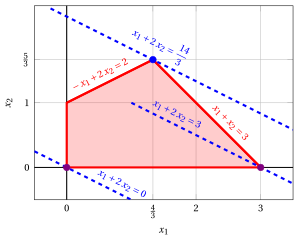
An optimal solution \({ \tilde{\boldsymbol x}}(\,LP\,)\) is:

\[ \tilde{x}_1=\dfrac{4}{3},~~\tilde{x}_2=\dfrac{5}{3} \]

the optimal value \(z(\, LP\,)\) is \(\dfrac{14}{3}.\)

In violet the first and the second vertex explored by the previous execution of the revised simplex algorithm (before reaching the optimal one depicted in blue).

In dashed blue, the contour lines of the objective function associated with the values taken in the three vertices.

Exercise 11.10: Revised simplex algorithm (P9)

Consider the following LP problem in canonical maximization form with \(n=2\) variables and \(m=2\) constraints:

\[ \begin{array}{rrrrrr} {\max} & {2}\, {x_1} & {+} & {x_2} \\[2ex] \text{subject to} & {-x_1} & {+} & {x_2} & {\le} & {1} \\[2ex] & {6}\, {x_1} & {+} & {4}\, {x_2} & {\le} & {39} \\[2ex] & {x_1,} & & {x_2} & {\ge} & {0} \end{array} \]

By introducing the slack variables, we get the following LP problem in standard maximization form with \(n+m=4\) variables and \(m=2\) constraints:

\[ \begin{array}{rrrrrrrrrr} {\max} & {2}\, {x_1} & {+} & {x_2} \\[2ex] \text{subject to} & {-x_1} & {+} & {x_2} & {+} & {x_3} & & & {=} & {1} \\[2ex] & {6}\, {x_1} & {+} & {4}\, {x_2} & & & {+} & {x_4} & {=} & {39} \\[2ex] & {x_1,} & & {x_2,} & & {x_3,} & & {x_4} & {\ge} & {0} \end{array} \]

Questions

• Execute the revised simplex algorithm to find an optimal solution of this LP problem using Bland's rule to select the pivot column and the pivot row.

Solution

We have:

\[ {\boldsymbol A}= \begin{pmatrix} -1 & 1 & 1 & 0\\ 6 & 4 & 0 & 1 \end{pmatrix} \quad {\boldsymbol b}= \begin{pmatrix} 1\\ 39 \end{pmatrix} \quad {\boldsymbol c}= \begin{pmatrix} 2\\ 1\\ 0\\ 0 \end{pmatrix} \quad {\boldsymbol x}= \begin{pmatrix} x_1 \\ x_2 \\ x_3 \\ x_4 \end{pmatrix} \]

• Initialization

  Since it is an LP problem in standard form obtained from an LP problem in canonical form with \(~{\boldsymbol b} \ge 0\) by adding the slack variables, the partition \(\pazocal{B}=\{3,4\}\) and \(\pazocal{N}=\{1,2\}\) is associated with the following basic feasible solution:

  \[ \begin{pmatrix} x_3 \\ x_4 \end{pmatrix} = \begin{pmatrix} 1\\ 39 \end{pmatrix} \text{ and } \begin{pmatrix} x_1 \\ x_2 \end{pmatrix} = \begin{pmatrix} 0\\ 0 \end{pmatrix} \]

• Iteration 1

  With \(\pazocal{B}= \{3,~~4\}\) and \(\pazocal{N}= \{1,~~2\}\), we have:

  \[ {\boldsymbol x}_{\pazocal{B}}= \begin{pmatrix} x_3 \\ x_4 \end{pmatrix} ~~ {\boldsymbol A}_{\pazocal{B}}= \begin{pmatrix} 1 & 0\\ 0 & 1 \end{pmatrix} ~~ {\boldsymbol c}_{\pazocal{B}}= \begin{pmatrix} 0\\ 0 \end{pmatrix} ~~ {{ \bar{\boldsymbol b}}}= \begin{pmatrix} 1\\ 39 \end{pmatrix} \]
  \[ {\boldsymbol x}_{\pazocal{N}}= \begin{pmatrix} x_1 \\ x_2 \end{pmatrix} ~~ {\boldsymbol A}_{\pazocal{N}}= \begin{pmatrix} -1 & 1\\ 6 & 4 \end{pmatrix} ~~ {\boldsymbol c}_{\pazocal{N}}= \begin{pmatrix} 2\\ 1 \end{pmatrix} \]

  Optimality check

  We solve \({\boldsymbol \pi} \; {\boldsymbol A}_{\pazocal{B}} = {\boldsymbol c}'_{\pazocal{B}}\) to compute \({\boldsymbol \pi} = {{{\boldsymbol c}'_{\pazocal{B}} \; {\boldsymbol A}_{\pazocal{B}}^{-1}}}\), first system of linear equations:

  \[\begin{equation*} \begin{cases} \begin{array}{rrrrr} {\pi_3} & & & {=} & {0} \\[2ex] & & {\pi_4} & {=} & {0} \end{array} \end{cases} \qquad {\boldsymbol \pi}= \begin{pmatrix} 0 & 0\\ \end{pmatrix} \end{equation*}\]

  We compute the basic feasible solution value \({\bar{z}} = {\boldsymbol \pi} \; {\boldsymbol b} = \begin{pmatrix} 0 & 0\\ \end{pmatrix} \begin{pmatrix} 1\\ 39 \end{pmatrix} = 0\)

  We compute the reduced costs \({{ \bar{\boldsymbol c}}'} = {{\boldsymbol c}'_{\pazocal{N}} - {\boldsymbol \pi} \; {\boldsymbol A}_{\pazocal{N}}}\):

  \[ {{ \bar{\boldsymbol c}}'} = \begin{pmatrix} 2 & 1\\ \end{pmatrix} - \begin{pmatrix} 0 & 0\\ \end{pmatrix} \begin{pmatrix} -1 & 1\\ 6 & 4 \end{pmatrix} = \underbrace{ \begin{pmatrix} 2 & 1\\ \end{pmatrix} }_{{c_{1}~~~c_{2}}} - \underbrace{ \begin{pmatrix} 0 & 0\\ \end{pmatrix} }_{{\boldsymbol \pi}\;{\boldsymbol A}_{1} ~~{\boldsymbol \pi}\;{\boldsymbol A}_{2}} = \underbrace{ \begin{pmatrix} 2 & 1\\ \end{pmatrix} }_{{\bar{c}_{1}~~~\bar{c}_{2}}} \]

  Not all reduced costs are non-positive then we perform a pivoting operation.

  Pivoting operation

  Since \({c}_{1} > {\boldsymbol \pi} \;{\boldsymbol A}_{1}\), \(x_1\) is the pivot column and we have \({\boldsymbol A}_{1} = \begin{pmatrix} -1\\ 6 \end{pmatrix}\)

  We solve \({\boldsymbol A}_{\pazocal{B}} \; {\boldsymbol d} = {\boldsymbol A}_{1}\) to compute \({\boldsymbol d}={ {\boldsymbol A}_{\pazocal{B}}^{-1}} {\boldsymbol A}_{1}\), second system of linear equations:

  \[\begin{equation*} \begin{cases} \begin{array}{rrrrr} {d_3} & & & {=} & {-1} \\[2ex] & & {d_4} & {=} & {6} \end{array} \end{cases} \qquad {\boldsymbol d}= \begin{pmatrix} -1\\ 6 \end{pmatrix} \end{equation*}\]

  We have to find the largest \(t\) such that \({{ \bar{\boldsymbol b}}} - t \; {{\boldsymbol d}} \ge 0\):

  \[ \begin{cases} \underbrace{1 -t \cdot \left( -1\right)\ge 0}_{x_3 \ge 0} \\[2ex] \underbrace{39 -t \cdot 6\ge 0}_{x_4 \ge 0} \end{cases} \qquad \begin{cases} t\ge -1 \\[2ex] t\le \dfrac{13}{2} \end{cases} \text{ then } t_{m}=\dfrac{13}{2} \]

  Accordingly the value of the pivot column becomes \(t_{m}\), i.e., \(x_1=\dfrac{13}{2}\). The value of \(x_4\) becomes zero and \(x_4\) is the pivot row. The other basic variables take values \({ \bar{\boldsymbol b}} - t_{m} \; {\boldsymbol d}\), then we have:

  \[ x_3 = 1 - \dfrac{13}{2} \cdot \left( -1\right) = \dfrac{15}{2} \]

• Iteration 2

  With \(\pazocal{B}= \{1,~~3\}\) and \(\pazocal{N}= \{2,~~4\}\), we have:

  \[ {\boldsymbol x}_{\pazocal{B}}= \begin{pmatrix} x_1 \\ x_3 \end{pmatrix} ~~ {\boldsymbol A}_{\pazocal{B}}= \begin{pmatrix} -1 & 1\\ 6 & 0 \end{pmatrix} ~~ {\boldsymbol c}_{\pazocal{B}}= \begin{pmatrix} 2\\ 0 \end{pmatrix} ~~ {{ \bar{\boldsymbol b}}}= \begin{pmatrix} \dfrac{13}{2}\\[2ex] \dfrac{15}{2} \end{pmatrix} \]
  \[ {\boldsymbol x}_{\pazocal{N}}= \begin{pmatrix} x_2 \\ x_4 \end{pmatrix} ~~ {\boldsymbol A}_{\pazocal{N}}= \begin{pmatrix} 1 & 0\\ 4 & 1 \end{pmatrix} ~~ {\boldsymbol c}_{\pazocal{N}}= \begin{pmatrix} 1\\ 0 \end{pmatrix} \]

  Optimality check

  We solve \({\boldsymbol \pi} \; {\boldsymbol A}_{\pazocal{B}} = {\boldsymbol c}'_{\pazocal{B}}\) to compute \({\boldsymbol \pi} = {{{\boldsymbol c}'_{\pazocal{B}} \; {\boldsymbol A}_{\pazocal{B}}^{-1}}}\), first system of linear equations:

  \[\begin{equation*} \begin{cases} \begin{array}{rrrrr} {-\pi_1} & {+} & {6}\, {\pi_3} & {=} & {2} \\[2ex] {\pi_1} & & & {=} & {0} \end{array} \end{cases} \qquad {\boldsymbol \pi}= \begin{pmatrix} 0 & \dfrac{1}{3}\\ \end{pmatrix} \end{equation*}\]

  We compute the basic feasible solution value \({\bar{z}} = {\boldsymbol \pi} \; {\boldsymbol b} = \begin{pmatrix} 0 & \dfrac{1}{3}\\ \end{pmatrix} \begin{pmatrix} 1\\ 39 \end{pmatrix} = 13\)

  We compute the reduced costs \({{ \bar{\boldsymbol c}}'} = {{\boldsymbol c}'_{\pazocal{N}} - {\boldsymbol \pi} \; {\boldsymbol A}_{\pazocal{N}}}\):

  \[ {{ \bar{\boldsymbol c}}'} = \begin{pmatrix} 1 & 0\\ \end{pmatrix} - \begin{pmatrix} 0 & \dfrac{1}{3}\\ \end{pmatrix} \begin{pmatrix} 1 & 0\\ 4 & 1 \end{pmatrix} = \underbrace{ \begin{pmatrix} 1 & 0\\ \end{pmatrix} }_{{c_{2}~~~c_{4}}} - \underbrace{ \begin{pmatrix} \dfrac{4}{3} & \dfrac{1}{3}\\ \end{pmatrix} }_{{\boldsymbol \pi}\;{\boldsymbol A}_{2} ~~{\boldsymbol \pi}\;{\boldsymbol A}_{4}} = \underbrace{ \begin{pmatrix} -\dfrac{1}{3} & -\dfrac{1}{3}\\ \end{pmatrix} }_{{\bar{c}_{2}~~~\bar{c}_{4}}} \]

  All reduced costs are non-positive, then the basic feasible solution

  \[ {\boldsymbol x}_{\pazocal{B}}= \begin{pmatrix} x_1 \\ x_3 \end{pmatrix}=\begin{pmatrix} \dfrac{13}{2}\\[2ex] \dfrac{15}{2} \end{pmatrix} \text{ and } {\boldsymbol x}_{\pazocal{N}}= \begin{pmatrix} x_2 \\ x_4 \end{pmatrix}=\begin{pmatrix} 0\\ 0 \end{pmatrix} \]

  is an optimal solution of the LP problem and \({\bar{z}} = 13\) is the optimal solution value.

Graphical solution:

The feasible region of the LP problem (in canonical form) is the polyhedron shaded in red:

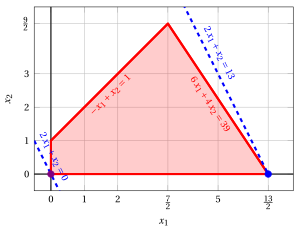
An optimal solution \({ \tilde{\boldsymbol x}}(\,LP\,)\) is:

\[ \tilde{x}_1=\dfrac{13}{2},~~\tilde{x}_2=0 \]

the optimal value \(z(\, LP\,)\) is \(13.\)

In violet the first vertex explored by the previous execution of the revised simplex algorithm (before reaching the optimal one depicted in blue).

In dashed blue, the contour lines of the objective function associated with the values taken in the two vertices.

Exercise 11.11: Revised simplex algorithm (P10)

Consider the following LP problem in canonical maximization form with \(n=2\) variables and \(m=3\) constraints:

\[ \begin{array}{rrrrrr} {\max} & {5}\, {x_1} & {+} & {2}\, {x_2} \\[2ex] \text{subject to} & {-x_1} & {+} & {3}\, {x_2} & {\le} & {12} \\[2ex] & {x_1} & {+} & {2}\, {x_2} & {\le} & {12} \\[2ex] & {3}\, {x_1} & {-} & {2}\, {x_2} & {\le} & {8} \\[2ex] & {x_1,} & & {x_2} & {\ge} & {0} \end{array} \]

By introducing the slack variables, we get the following LP problem in standard maximization form with \(n+m=5\) variables and \(m=3\) constraints:

\[ \begin{array}{rrrrrrrrrrrr} {\max} & {5}\, {x_1} & {+} & {2}\, {x_2} \\[2ex] \text{subject to} & {-x_1} & {+} & {3}\, {x_2} & {+} & {x_3} & & & & & {=} & {12} \\[2ex] & {x_1} & {+} & {2}\, {x_2} & & & {+} & {x_4} & & & {=} & {12} \\[2ex] & {3}\, {x_1} & {-} & {2}\, {x_2} & & & & & {+} & {x_5} & {=} & {8} \\[2ex] & {x_1,} & & {x_2,} & & {x_3,} & & {x_4,} & & {x_5} & {\ge} & {0} \end{array} \]

Questions

• Execute the revised simplex algorithm to find an optimal solution of this LP problem using Bland's rule to select the pivot column and the pivot row.

Solution

We have:

\[ {\boldsymbol A}= \begin{pmatrix} -1 & 3 & 1 & 0 & 0\\ 1 & 2 & 0 & 1 & 0\\ 3 & -2 & 0 & 0 & 1 \end{pmatrix} \quad {\boldsymbol b}= \begin{pmatrix} 12\\ 12\\ 8 \end{pmatrix} \quad {\boldsymbol c}= \begin{pmatrix} 5\\ 2\\ 0\\ 0\\ 0 \end{pmatrix} \quad {\boldsymbol x}= \begin{pmatrix} x_1 \\ x_2 \\ x_3 \\ x_4 \\ x_5 \end{pmatrix} \]

• Initialization

  Since it is an LP problem in standard form obtained from an LP problem in canonical form with \(~{\boldsymbol b} \ge 0\) by adding the slack variables, the partition \(\pazocal{B}=\{3,4,5\}\) and \(\pazocal{N}=\{1,2\}\) is associated with the following basic feasible solution:

  \[ \begin{pmatrix} x_3 \\ x_4 \\ x_5 \end{pmatrix} = \begin{pmatrix} 12\\ 12\\ 8 \end{pmatrix} \text{ and } \begin{pmatrix} x_1 \\ x_2 \end{pmatrix} = \begin{pmatrix} 0\\ 0 \end{pmatrix} \]

• Iteration 1

  With \(\pazocal{B}= \{3,~~4,~~5\}\) and \(\pazocal{N}= \{1,~~2\}\), we have:

  \[ {\boldsymbol x}_{\pazocal{B}}= \begin{pmatrix} x_3 \\ x_4 \\ x_5 \end{pmatrix} ~~ {\boldsymbol A}_{\pazocal{B}}= \begin{pmatrix} 1 & 0 & 0\\ 0 & 1 & 0\\ 0 & 0 & 1 \end{pmatrix} ~~ {\boldsymbol c}_{\pazocal{B}}= \begin{pmatrix} 0\\ 0\\ 0 \end{pmatrix} ~~ {{ \bar{\boldsymbol b}}}= \begin{pmatrix} 12\\ 12\\ 8 \end{pmatrix} \]
  \[ {\boldsymbol x}_{\pazocal{N}}= \begin{pmatrix} x_1 \\ x_2 \end{pmatrix} ~~ {\boldsymbol A}_{\pazocal{N}}= \begin{pmatrix} -1 & 3\\ 1 & 2\\ 3 & -2 \end{pmatrix} ~~ {\boldsymbol c}_{\pazocal{N}}= \begin{pmatrix} 5\\ 2 \end{pmatrix} \]

  Optimality check

  We solve \({\boldsymbol \pi} \; {\boldsymbol A}_{\pazocal{B}} = {\boldsymbol c}'_{\pazocal{B}}\) to compute \({\boldsymbol \pi} = {{{\boldsymbol c}'_{\pazocal{B}} \; {\boldsymbol A}_{\pazocal{B}}^{-1}}}\), first system of linear equations:

  \[\begin{equation*} \begin{cases} \begin{array}{rrrrrrr} {\pi_3} & & & & & {=} & {0} \\[2ex] & & {\pi_4} & & & {=} & {0} \\[2ex] & & & & {\pi_5} & {=} & {0} \end{array} \end{cases} \qquad {\boldsymbol \pi}= \begin{pmatrix} 0 & 0 & 0\\ \end{pmatrix} \end{equation*}\]

  We compute the basic feasible solution value \({\bar{z}} = {\boldsymbol \pi} \; {\boldsymbol b} = \begin{pmatrix} 0 & 0 & 0\\ \end{pmatrix} \begin{pmatrix} 12\\ 12\\ 8 \end{pmatrix} = 0\)

  We compute the reduced costs \({{ \bar{\boldsymbol c}}'} = {{\boldsymbol c}'_{\pazocal{N}} - {\boldsymbol \pi} \; {\boldsymbol A}_{\pazocal{N}}}\):

  \[ \begin{aligned} {{ \bar{\boldsymbol c}}'} &= \begin{pmatrix} 5 & 2\\ \end{pmatrix} - \begin{pmatrix} 0 & 0 & 0\\ \end{pmatrix} \begin{pmatrix} -1 & 3\\ 1 & 2\\ 3 & -2 \end{pmatrix} \\[1ex] &= \underbrace{ \begin{pmatrix} 5 & 2\\ \end{pmatrix} }_{{c_{1}~~~c_{2}}} - \underbrace{ \begin{pmatrix} 0 & 0\\ \end{pmatrix} }_{{\boldsymbol \pi}\;{\boldsymbol A}_{1} ~~{\boldsymbol \pi}\;{\boldsymbol A}_{2}} = \underbrace{ \begin{pmatrix} 5 & 2\\ \end{pmatrix} }_{{\bar{c}_{1}~~~\bar{c}_{2}}} \end{aligned} \]

  Not all reduced costs are non-positive then we perform a pivoting operation.

  Pivoting operation

  Since \({c}_{1} > {\boldsymbol \pi} \;{\boldsymbol A}_{1}\), \(x_1\) is the pivot column and we have \({\boldsymbol A}_{1} = \begin{pmatrix} -1\\ 1\\ 3 \end{pmatrix}\)

  We solve \({\boldsymbol A}_{\pazocal{B}} \; {\boldsymbol d} = {\boldsymbol A}_{1}\) to compute \({\boldsymbol d}={ {\boldsymbol A}_{\pazocal{B}}^{-1}} {\boldsymbol A}_{1}\), second system of linear equations:

  \[\begin{equation*} \begin{cases} \begin{array}{rrrrrrr} {d_3} & & & & & {=} & {-1} \\[2ex] & & {d_4} & & & {=} & {1} \\[2ex] & & & & {d_5} & {=} & {3} \end{array} \end{cases} \qquad {\boldsymbol d}= \begin{pmatrix} -1\\ 1\\ 3 \end{pmatrix} \end{equation*}\]

  We have to find the largest \(t\) such that \({{ \bar{\boldsymbol b}}} - t \; {{\boldsymbol d}} \ge 0\):

  \[ \begin{cases} \underbrace{12 -t \cdot \left( -1\right)\ge 0}_{x_3 \ge 0} \\[2ex] \underbrace{12 -t \cdot 1\ge 0}_{x_4 \ge 0} \\[2ex] \underbrace{8 -t \cdot 3\ge 0}_{x_5 \ge 0} \end{cases} \qquad \begin{cases} t\ge -12 \\[2ex] t\le 12 \\[2ex] t\le \dfrac{8}{3} \end{cases} \text{ then } t_{m}=\dfrac{8}{3} \]

  Accordingly the value of the pivot column becomes \(t_{m}\), i.e., \(x_1=\dfrac{8}{3}\). The value of \(x_5\) becomes zero and \(x_5\) is the pivot row. The other basic variables take values \({ \bar{\boldsymbol b}} - t_{m} \; {\boldsymbol d}\), then we have:

  \[ \begin{aligned} x_3 &= 12 - \dfrac{8}{3} \cdot \left( -1\right) = \dfrac{44}{3} \\[2ex] x_4 &= 12 - \dfrac{8}{3} \cdot 1 = \dfrac{28}{3} \end{aligned} \]

• Iteration 2

  With \(\pazocal{B}= \{1,~~3,~~4\}\) and \(\pazocal{N}= \{2,~~5\}\), we have:

  \[ {\boldsymbol x}_{\pazocal{B}}= \begin{pmatrix} x_1 \\ x_3 \\ x_4 \end{pmatrix} ~~ {\boldsymbol A}_{\pazocal{B}}= \begin{pmatrix} -1 & 1 & 0\\ 1 & 0 & 1\\ 3 & 0 & 0 \end{pmatrix} ~~ {\boldsymbol c}_{\pazocal{B}}= \begin{pmatrix} 5\\ 0\\ 0 \end{pmatrix} ~~ {{ \bar{\boldsymbol b}}}= \begin{pmatrix} \dfrac{8}{3}\\[2ex] \dfrac{44}{3}\\[2ex] \dfrac{28}{3} \end{pmatrix} \]
  \[ {\boldsymbol x}_{\pazocal{N}}= \begin{pmatrix} x_2 \\ x_5 \end{pmatrix} ~~ {\boldsymbol A}_{\pazocal{N}}= \begin{pmatrix} 3 & 0\\ 2 & 0\\ -2 & 1 \end{pmatrix} ~~ {\boldsymbol c}_{\pazocal{N}}= \begin{pmatrix} 2\\ 0 \end{pmatrix} \]

  Optimality check

  We solve \({\boldsymbol \pi} \; {\boldsymbol A}_{\pazocal{B}} = {\boldsymbol c}'_{\pazocal{B}}\) to compute \({\boldsymbol \pi} = {{{\boldsymbol c}'_{\pazocal{B}} \; {\boldsymbol A}_{\pazocal{B}}^{-1}}}\), first system of linear equations:

  \[\begin{equation*} \begin{cases} \begin{array}{rrrrrrr} {-\pi_1} & {+} & {\pi_3} & {+} & {3}\, {\pi_4} & {=} & {5} \\[2ex] {\pi_1} & & & & & {=} & {0} \\[2ex] & & {\pi_3} & & & {=} & {0} \end{array} \end{cases} \qquad {\boldsymbol \pi}= \begin{pmatrix} 0 & 0 & \dfrac{5}{3}\\ \end{pmatrix} \end{equation*}\]

  We compute the basic feasible solution value \({\bar{z}} = {\boldsymbol \pi} \; {\boldsymbol b} = \begin{pmatrix} 0 & 0 & \dfrac{5}{3}\\ \end{pmatrix} \begin{pmatrix} 12\\ 12\\ 8 \end{pmatrix} = \dfrac{40}{3}\)

  We compute the reduced costs \({{ \bar{\boldsymbol c}}'} = {{\boldsymbol c}'_{\pazocal{N}} - {\boldsymbol \pi} \; {\boldsymbol A}_{\pazocal{N}}}\):

  \[ \begin{aligned} {{ \bar{\boldsymbol c}}'} &= \begin{pmatrix} 2 & 0\\ \end{pmatrix} - \begin{pmatrix} 0 & 0 & \dfrac{5}{3}\\ \end{pmatrix} \begin{pmatrix} 3 & 0\\ 2 & 0\\ -2 & 1 \end{pmatrix} \\[1ex] &= \underbrace{ \begin{pmatrix} 2 & 0\\ \end{pmatrix} }_{{c_{2}~~~c_{5}}} - \underbrace{ \begin{pmatrix} -\dfrac{10}{3} & \dfrac{5}{3}\\ \end{pmatrix} }_{{\boldsymbol \pi}\;{\boldsymbol A}_{2} ~~{\boldsymbol \pi}\;{\boldsymbol A}_{5}} = \underbrace{ \begin{pmatrix} \dfrac{16}{3} & -\dfrac{5}{3}\\ \end{pmatrix} }_{{\bar{c}_{2}~~~\bar{c}_{5}}} \end{aligned} \]

  Not all reduced costs are non-positive then we perform a pivoting operation.

  Pivoting operation

  Since \({c}_{2} > {\boldsymbol \pi} \;{\boldsymbol A}_{2}\), \(x_2\) is the pivot column and we have \({\boldsymbol A}_{2} = \begin{pmatrix} 3\\ 2\\ -2 \end{pmatrix}\)

  We solve \({\boldsymbol A}_{\pazocal{B}} \; {\boldsymbol d} = {\boldsymbol A}_{2}\) to compute \({\boldsymbol d}={ {\boldsymbol A}_{\pazocal{B}}^{-1}} {\boldsymbol A}_{2}\), second system of linear equations:

  \[\begin{equation*} \begin{cases} \begin{array}{rrrrrrr} {-d_1} & {+} & {d_3} & & & {=} & {3} \\[2ex] {d_1} & & & {+} & {d_4} & {=} & {2} \\[2ex] {3}\, {d_1} & & & & & {=} & {-2} \end{array} \end{cases} \qquad {\boldsymbol d}= \begin{pmatrix} -\dfrac{2}{3}\\[2ex] \dfrac{7}{3}\\[2ex] \dfrac{8}{3} \end{pmatrix} \end{equation*}\]

  We have to find the largest \(t\) such that \({{ \bar{\boldsymbol b}}} - t \; {{\boldsymbol d}} \ge 0\):

  \[ \begin{cases} \underbrace{\dfrac{8}{3} -t \cdot \left( -\dfrac{2}{3}\right)\ge 0}_{x_1 \ge 0} \\[2ex] \underbrace{\dfrac{44}{3} -t \cdot \dfrac{7}{3}\ge 0}_{x_3 \ge 0} \\[2ex] \underbrace{\dfrac{28}{3} -t \cdot \dfrac{8}{3}\ge 0}_{x_4 \ge 0} \end{cases} \qquad \begin{cases} t\ge -4 \\[2ex] t\le \dfrac{44}{7} \\[2ex] t\le \dfrac{7}{2} \end{cases} \text{ then } t_{m}=\dfrac{7}{2} \]

  Accordingly the value of the pivot column becomes \(t_{m}\), i.e., \(x_2=\dfrac{7}{2}\). The value of \(x_4\) becomes zero and \(x_4\) is the pivot row. The other basic variables take values \({ \bar{\boldsymbol b}} - t_{m} \; {\boldsymbol d}\), then we have:

  \[ \begin{aligned} x_1 &= \dfrac{8}{3} - \dfrac{7}{2} \cdot \left( -\dfrac{2}{3}\right) = 5 \\[2ex] x_3 &= \dfrac{44}{3} - \dfrac{7}{2} \cdot \dfrac{7}{3} = \dfrac{13}{2} \end{aligned} \]

• Iteration 3

  With \(\pazocal{B}= \{1,~~2,~~3\}\) and \(\pazocal{N}= \{4,~~5\}\), we have:

  \[ {\boldsymbol x}_{\pazocal{B}}= \begin{pmatrix} x_1 \\ x_2 \\ x_3 \end{pmatrix} ~~ {\boldsymbol A}_{\pazocal{B}}= \begin{pmatrix} -1 & 3 & 1\\ 1 & 2 & 0\\ 3 & -2 & 0 \end{pmatrix} ~~ {\boldsymbol c}_{\pazocal{B}}= \begin{pmatrix} 5\\ 2\\ 0 \end{pmatrix} ~~ {{ \bar{\boldsymbol b}}}= \begin{pmatrix} 5\\[2ex] \dfrac{7}{2}\\[2ex] \dfrac{13}{2} \end{pmatrix} \]
  \[ {\boldsymbol x}_{\pazocal{N}}= \begin{pmatrix} x_4 \\ x_5 \end{pmatrix} ~~ {\boldsymbol A}_{\pazocal{N}}= \begin{pmatrix} 0 & 0\\ 1 & 0\\ 0 & 1 \end{pmatrix} ~~ {\boldsymbol c}_{\pazocal{N}}= \begin{pmatrix} 0\\ 0 \end{pmatrix} \]

  Optimality check

  We solve \({\boldsymbol \pi} \; {\boldsymbol A}_{\pazocal{B}} = {\boldsymbol c}'_{\pazocal{B}}\) to compute \({\boldsymbol \pi} = {{{\boldsymbol c}'_{\pazocal{B}} \; {\boldsymbol A}_{\pazocal{B}}^{-1}}}\), first system of linear equations:

  \[\begin{equation*} \begin{cases} \begin{array}{rrrrrrr} {-\pi_1} & {+} & {\pi_2} & {+} & {3}\, {\pi_3} & {=} & {5} \\[2ex] {3}\, {\pi_1} & {+} & {2}\, {\pi_2} & {-} & {2}\, {\pi_3} & {=} & {2} \\[2ex] {\pi_1} & & & & & {=} & {0} \end{array} \end{cases} \qquad {\boldsymbol \pi}= \begin{pmatrix} 0 & 2 & 1\\ \end{pmatrix} \end{equation*}\]

  We compute the basic feasible solution value \({\bar{z}} = {\boldsymbol \pi} \; {\boldsymbol b} = \begin{pmatrix} 0 & 2 & 1\\ \end{pmatrix} \begin{pmatrix} 12\\ 12\\ 8 \end{pmatrix} = 32\)

  We compute the reduced costs \({{ \bar{\boldsymbol c}}'} = {{\boldsymbol c}'_{\pazocal{N}} - {\boldsymbol \pi} \; {\boldsymbol A}_{\pazocal{N}}}\):

  \[ \begin{aligned} {{ \bar{\boldsymbol c}}'} &= \begin{pmatrix} 0 & 0\\ \end{pmatrix} - \begin{pmatrix} 0 & 2 & 1\\ \end{pmatrix} \begin{pmatrix} 0 & 0\\ 1 & 0\\ 0 & 1 \end{pmatrix} \\[1ex] &= \underbrace{ \begin{pmatrix} 0 & 0\\ \end{pmatrix} }_{{c_{4}~~~c_{5}}} - \underbrace{ \begin{pmatrix} 2 & 1\\ \end{pmatrix} }_{{\boldsymbol \pi}\;{\boldsymbol A}_{4} ~~{\boldsymbol \pi}\;{\boldsymbol A}_{5}} = \underbrace{ \begin{pmatrix} -2 & -1\\ \end{pmatrix} }_{{\bar{c}_{4}~~~\bar{c}_{5}}} \end{aligned} \]

  All reduced costs are non-positive, then the basic feasible solution

  \[ {\boldsymbol x}_{\pazocal{B}}= \begin{pmatrix} x_1 \\ x_2 \\ x_3 \end{pmatrix}=\begin{pmatrix} 5\\[2ex] \dfrac{7}{2}\\[2ex] \dfrac{13}{2} \end{pmatrix} \text{ and } {\boldsymbol x}_{\pazocal{N}}= \begin{pmatrix} x_4 \\ x_5 \end{pmatrix}=\begin{pmatrix} 0\\ 0 \end{pmatrix} \]

  is an optimal solution of the LP problem and \({\bar{z}} = 32\) is the optimal solution value.

Graphical solution:

The feasible region of the LP problem (in canonical form) is the polyhedron shaded in red:

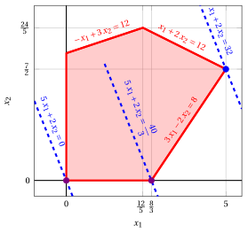
An optimal solution \({ \tilde{\boldsymbol x}}(\,LP\,)\) is:

\[ \tilde{x}_1=5,~~\tilde{x}_2=\dfrac{7}{2} \]

the optimal value \(z(\, LP\,)\) is \(32.\)

In violet the first and the second vertex explored by the previous execution of the revised simplex algorithm (before reaching the optimal one depicted in blue).

In dashed blue, the contour lines of the objective function associated with the values taken in the three vertices.

Exercise 11.12: First phase of the revised simplex algorithm (P21)

Consider the following LP problem in canonical maximization form with \(n=2\) variables and \(m=3\) constraints:

\[ \begin{array}{rrrrrrrrrrrrr} {\max} & \, {x_1} & {+} & {2} \, {x_2} \\[2ex] \text{subject to} & {- }\, {x_1} & {-} & \, {x_2} & {\le} & {-2} \\[2ex] & {4} \, {x_1} & {-} & {2} \, {x_2} & {\le} & {7} \\[2ex] & {x_1} & {+} & {5} \, {x_2} & {\le} & {21} \\[2ex] & {x_1,} & & {x_2} & { \ge} & {0 } \end{array} \]

Questions

1. Solve the first phase of the simplex algorithm using Bland's rule to select the pivot column and the pivot row.

2. Starting from the basic feasible solution obtained in the previous question, solve this LP problem using the revised simplex algorithm and Bland's rule to select the pivot column and the pivot row.

Solution

1. We write the auxiliary problem:

   \[ \begin{array}{rcrcrcrcrcrcrcr} {\max} & {-} & {x_0} & & & & & & & & \\[2ex] \text{subject to} & {-} & {x_0} & {- } & \, {x_1} & {-} & \, {x_2} & {+} & \, {x_3} & & & & & {=} & {-2} \\[2ex] & {-} & {x_0} & {+} & {4} \, {x_1} & {-} & {2} \, {x_2} & & & {+} & \, {x_4} & & & {=} & {7} \\[2ex] & {-} & {x_0} & {+} & {x_1} & {+} & {5} \, {x_2} & & & & & {+} & \, {x_5} & {=} & {21} \\[2ex] & & {x_0,} & & {x_1,} & & {x_2,} & & {x_3,} & & {x_4,} & & \, {x_5} & { \ge} & {0 } \end{array} \]

   Now there are \(n + m + 1 = 6\) variables and \(m = 3\) constraints. We have:

   \[ {\boldsymbol A}= \begin{pmatrix} -1 & -1 & -1 & 1 & 0 & 0\\[2ex] -1 & 4 & -2 & 0 & 1 & 0\\[2ex] -1 & 1 & 5 & 0 & 0 & 1\\ \end{pmatrix} \quad {\boldsymbol b}= \begin{pmatrix} -2 \\[2ex] 7 \\[2ex] 21 \\ \end{pmatrix} \quad {\boldsymbol c}= \begin{pmatrix} -1 \\ 0 \\ 0 \\ 0 \\ 0 \\ 0 \\ \end{pmatrix} \quad {\boldsymbol x}= \begin{pmatrix} x_{0} \\ x_{1} \\ x_{2} \\ x_{3} \\ x_{4} \\ x_{5} \\ \end{pmatrix} \]

   • Initialization

     We consider \(\pazocal{B}= \{3,~~4,~~5\}\) and \(\pazocal{N}= \{0,~~1,~~2\}\), we have:

     \[ {\boldsymbol x}_{\pazocal{B}}= \begin{pmatrix} x_3 \\ x_4 \\ x_5 \\ \end{pmatrix} ~~ {\boldsymbol A}_{\pazocal{B}}= \begin{pmatrix} 1 & 0 & 0\\ 0 & 1 & 0\\ 0 & 0 & 1\\ \end{pmatrix} ~~ {\boldsymbol c}_{\pazocal{B}}= \begin{pmatrix} 0 \\ 0 \\ 0 \\ \end{pmatrix} ~~ {{ \bar{\boldsymbol b}}}=\begin{pmatrix} -2 \\ 7 \\ 21 \\ \end{pmatrix} \]
     \[ {\boldsymbol x}_{\pazocal{N}}= \begin{pmatrix} x_0 \\ x_1 \\ x_2 \\ \end{pmatrix} ~~ {\boldsymbol A}_{\pazocal{N}}= \begin{pmatrix} -1 & -1 & -1\\ -1 & 4 & -2 \\ -1 & 1 & 5 \\ \end{pmatrix} ~~ {\boldsymbol c}_{\pazocal{N}}= \begin{pmatrix} -1 \\ 0 \\ 0 \\ \end{pmatrix} \]

     First Pivoting operation

     The variable \(x_0\) enters the basis and \(x_3\) leaves the basis, since \(x_3\) is the slack variable associated with the most negative RHS (also the only negative one). We have \(x_0 = - b_1 = 2\).

     The other basic variables \(x_j\) with \(j \in \pazocal B\) take values \(x_j ~ = ~ {b}_j - b_1\,\), then we have:

     \[ x_4= 7 - (- 2) = 9 \]
     \[ x_5= 21 - (- 2) = 23 \]

     The new basic variables are \({\boldsymbol x}_{\pazocal{B}}=\begin{pmatrix} x_0 \\ x_4 \\ x_5 \\ \end{pmatrix}\). The basic feasible solution is \({{ \bar{\boldsymbol b}}}=\begin{pmatrix} 2 \\ 9 \\ 23 \\ \end{pmatrix}\)

   • Iteration 1

     With \(\pazocal{B}= \{0,~~4,~~5\}\) and \(\pazocal{N}= \{1,~~2,~~3\}\), we have:

     \[ {\boldsymbol x}_{\pazocal{B}}= \begin{pmatrix} x_0 \\ x_4 \\ x_5 \\ \end{pmatrix} ~~ {\boldsymbol A}_{\pazocal{B}}= \begin{pmatrix} -1 & 0 & 0\\ -1 & 1 & 0\\ -1 & 0 & 1\\ \end{pmatrix} ~~ {\boldsymbol c}_{\pazocal{B}}= \begin{pmatrix} -1 \\ 0 \\ 0 \\ \end{pmatrix} ~~ {{ \bar{\boldsymbol b}}}=\begin{pmatrix} 2 \\ 9 \\ 23 \\ \end{pmatrix} \]
     \[ {\boldsymbol x}_{\pazocal{N}}= \begin{pmatrix} x_1 \\ x_2 \\ x_3 \\ \end{pmatrix} ~~ {\boldsymbol A}_{\pazocal{N}}= \begin{pmatrix} -1 & -1 & 1\\ 4 & -2 & 0\\ 1 & 5 & 0\\ \end{pmatrix} ~~ {\boldsymbol c}_{\pazocal{N}}= \begin{pmatrix} 0 \\ 0 \\ 0 \\ \end{pmatrix} \]

     Optimality check

     We solve \({\boldsymbol \pi} \; {\boldsymbol A}_{\pazocal{B}} = {\boldsymbol c}'_{\pazocal{B}}\) to compute \({\boldsymbol \pi} = {{{\boldsymbol c}'_{\pazocal{B}} \; {\boldsymbol A}_{\pazocal{B}}^{-1}}}\), first system of linear equations:

     \[\begin{equation*} \begin{cases} \begin{array}{rrrrrrrrrrrrr} {-} & {\pi_0} & {-} & {\, \pi_4} & {-} & { \pi_5} & {=} & {-1} \\[2ex] & & & {\pi_4} & & & {=} & {0} \\[2ex] & & & & & {\pi_5} & {=} & {0} \end{array} \end{cases} \qquad {\boldsymbol \pi}= \begin{pmatrix} 1 & 0 & 0\\ \end{pmatrix} \end{equation*}\]

     We compute the basic feasible solution value \({\bar{z}} = {\boldsymbol \pi} \; {\boldsymbol b} = \begin{pmatrix} 1 & 0 & 0 \\ \end{pmatrix} \begin{pmatrix} -2 \\ 7 \\ 21 \\ \end{pmatrix} = -2\)

     We compute the reduced costs \({{ \bar{\boldsymbol c}}'} = {{\boldsymbol c}'_{\pazocal{N}} - {\boldsymbol \pi} \; {\boldsymbol A}_{\pazocal{N}}}\):

     \[ \begin{aligned} {{ \bar{\boldsymbol c}}'} &= \begin{pmatrix} 0 & 0 & 0 \\ \end{pmatrix} - \begin{pmatrix} 1 & 0 & 0 \\ \end{pmatrix} \begin{pmatrix} -1 & -1 & 1\\ 4 & -2 & 0\\ 1 & 5 & 0\\ \end{pmatrix} \\[1ex] &= \underbrace{ \begin{pmatrix} 0 & 0 & 0 \\ \end{pmatrix} }_{{c_{1}~~~c_{2}~~~c_{3}}} - \underbrace{ \begin{pmatrix} -1 & -1 & 1\\ \end{pmatrix} }_{{\boldsymbol \pi}\;{\boldsymbol A}_{1} ~~{\boldsymbol \pi}\;{\boldsymbol A}_{2} ~~{\boldsymbol \pi}\;{\boldsymbol A}_{3}} = \underbrace{ \begin{pmatrix} 1 & 1 & -1 \\ \end{pmatrix} }_{{\bar{c}_{1}~~~~\bar{c}_{2}~~~~\bar{c}_{3}}} \end{aligned} \]

     Not all reduced costs are non-positive then we perform a pivoting operation.

     Pivoting operation

     Since \({c}_1 > {\boldsymbol \pi} \;{\boldsymbol A}_{1}\), \(x_1\) is the pivot column and we have \({\boldsymbol A}_{1} = \begin{pmatrix} -1 \\ 4 \\ 1 \end{pmatrix}\)

     We solve \({\boldsymbol A}_{\pazocal{B}} \; {\boldsymbol d} = {\boldsymbol A}_{1}\) to compute \({\boldsymbol d}={ {\boldsymbol A}_{\pazocal{B}}^{-1}} {\boldsymbol A}_{1}\), second system of linear equations:

     \[\begin{equation*} \begin{cases} \begin{array}{rrrrrrrrrrrrr} {-} & {d_0} & & & & & {=} & {-1} \\[2ex] {-} & {d_0} & + & {d_4} & & & {=} & {4} \\[2ex] {-} & {d_0} & & & + & {d_5} & {=} & {1} \end{array} \end{cases} \qquad {\boldsymbol d}= \begin{pmatrix} 1 \\ 5 \\ 2 \\ \end{pmatrix} \end{equation*}\]

     We have to find the largest \(t\) such that \({{ \bar{\boldsymbol b}}} - t \; {{\boldsymbol d}} \ge 0\):

     \[ \begin{cases} \underbrace{2 -t \cdot \left( 1\right)\ge 0}_{x_0 \ge 0} \\[1ex] \underbrace{9 -t \cdot \left( 5\right)\ge 0}_{x_4 \ge 0} \\[1ex] \underbrace{23 -t \cdot \left( 2\right)\ge 0}_{x_5 \ge 0} \\ \end{cases} \qquad \begin{cases} t\le 2 \\[1ex] t\le \frac{9}{5} \\[1ex] t \le \frac{23}{2} \\ \end{cases} \text{ then } t_{m}=\frac{9}{5} \]

     Accordingly, the value of the pivot column becomes \(t_{m}\), i.e., \(x_1=\frac{9}{5}\). The value of \(x_4\) becomes zero and \(x_4\) is the pivot row. The other basic variables take values \({ \bar{\boldsymbol b}} - t_{m} \; {\boldsymbol d}\), then we have:

     \[ x_0= 2 - \frac{9}{5} \cdot \left( 1\right)= \frac{1}{5} \]
     \[ x_5= 23 - \frac{9}{5} \cdot \left( 2\right)= \frac{97}{5} \]

   • Iteration 2

     With \(\pazocal{B}= \{0,~~1,~~5\}\) and \(\pazocal{N}= \{2,~~3,~~4 \}\), we have:

     \[ {\boldsymbol x}_{\pazocal{B}}= \begin{pmatrix} x_0 \\ x_1 \\ x_5 \\ \end{pmatrix} ~~ {\boldsymbol A}_{\pazocal{B}}= \begin{pmatrix} -1 & -1 & 0\\ -1 & 4 & 0\\ -1 & 1 & 1\\ \end{pmatrix} ~~ {\boldsymbol c}_{\pazocal{B}}= \begin{pmatrix} -1 \\ 0 \\ 0 \\ \end{pmatrix} ~~ {{ \bar{\boldsymbol b}}}=\begin{pmatrix} \frac{1}{5} \\[1.5ex] \frac{9}{5} \\[1.5ex] \frac{97}{5} \\ \end{pmatrix} \]
     \[ {\boldsymbol x}_{\pazocal{N}}= \begin{pmatrix} x_2 \\ x_3 \\ x_4 \\ \end{pmatrix} ~~ {\boldsymbol A}_{\pazocal{N}}= \begin{pmatrix} -1 & 1 & 0 \\ -2 & 0 & 1 \\ 5 & 0 & 0 \\ \end{pmatrix} ~~ {\boldsymbol c}_{\pazocal{N}}= \begin{pmatrix} 0 \\ 0 \\ 0 \\ \end{pmatrix} \]

     Optimality check

     We solve \({\boldsymbol \pi} \; {\boldsymbol A}_{\pazocal{B}} = {\boldsymbol c}'_{\pazocal{B}}\) to compute \({\boldsymbol \pi} = {{{\boldsymbol c}'_{\pazocal{B}} \; {\boldsymbol A}_{\pazocal{B}}^{-1}}}\), first system of linear equations:

     \[\begin{equation*} \begin{cases} \begin{array}{rrrrrrrrrrrrr} {-} & {\pi_0} & {-} & {\, \pi_1} & {-} & { \pi_5} & {=} & {-1} \\[2ex] {-} & {\pi_0} & + & {4\, \pi_1} & & & {=} & {0} \\[2ex] & & & & & { \pi_5} & {=} & {0} \end{array} \end{cases} \qquad {\boldsymbol \pi}= \begin{pmatrix} \frac{4}{5} & \frac{1}{5} & 0\\ \end{pmatrix} \end{equation*}\]

     We compute the basic feasible solution value \({\bar{z}} = {\boldsymbol \pi} \; {\boldsymbol b} = \begin{pmatrix} \frac{4}{5} & \frac{1}{5} & 0 \\ \end{pmatrix} \begin{pmatrix} -2 \\ 7 \\ 21 \\ \end{pmatrix} = -\frac{1}{5}\)

     We compute the reduced costs \({{ \bar{\boldsymbol c}}'} = {{\boldsymbol c}'_{\pazocal{N}} - {\boldsymbol \pi} \; {\boldsymbol A}_{\pazocal{N}}}\):

     \[ \begin{aligned} {{ \bar{\boldsymbol c}}'} &= \begin{pmatrix} 0 & 0 & 0 \\ \end{pmatrix} - \begin{pmatrix} \frac{4}{5} & \frac{1}{5} & 0\\ \end{pmatrix} \begin{pmatrix} -1 & 1 & 0 \\ -2 & 0 & 1 \\ 5 & 0 & 0 \\ \end{pmatrix} \\[1ex] &= \underbrace{ \begin{pmatrix} 0 & 0 & 0 \\ \end{pmatrix} }_{{c_{2}~~~c_{3}~~~c_{4}}} - \underbrace{ \begin{pmatrix} -\frac{6}{5} & \frac{4}{5} & \frac{1}{5} \\ \end{pmatrix} }_{{\boldsymbol \pi}\;{\boldsymbol A}_{2} ~~{\boldsymbol \pi}\;{\boldsymbol A}_{3} ~~{\boldsymbol \pi}\;{\boldsymbol A}_{4}} = \underbrace{ \begin{pmatrix} \frac{6}{5} & -\frac{4}{5} & -\frac{1}{5} \end{pmatrix} }_{{\bar{c}_{2}~~~~~~\bar{c}_{3}~~~~~~~\bar{c}_{4}}} \end{aligned} \]

     Not all reduced costs are non-positive then we perform a pivoting operation.

     Pivoting operation

     Since \({c}_2 > {\boldsymbol \pi} \;{\boldsymbol A}_{2}\), \(x_2\) is the pivot column and we have \({\boldsymbol A}_{2} = \begin{pmatrix} -1 \\ -2 \\ 5 \end{pmatrix}\)

     We solve \({\boldsymbol A}_{\pazocal{B}} \; {\boldsymbol d} = {\boldsymbol A}_{2}\) to compute \({\boldsymbol d}={ {\boldsymbol A}_{\pazocal{B}}^{-1}} {\boldsymbol A}_{2}\), second system of linear equations:

     \[\begin{equation*} \begin{cases} \begin{array}{rrrrrrrrrrrrr} {-} & { d_0} & {-} & {d_1} & & & {=} & {-1} \\[2ex] {-} & {d_0} & {+} & {4\, d_1} & & & {=} & {-2} \\[2ex] {-} & { d_0} & + & {d_1} & {+} & { d_5} & {=} & {5} \end{array} \end{cases} \qquad {\boldsymbol d}= \begin{pmatrix} \frac{6}{5} \\[1.5ex] -\frac{1}{5} \\[1.5ex] \frac{32}{5} \\ \end{pmatrix} \end{equation*}\]

     We have to find the largest \(t\) such that \({{ \bar{\boldsymbol b}}} - t \; {{\boldsymbol d}} \ge 0\):

     \[ \begin{cases} \underbrace{\frac{1}{5} -t \cdot \left( \frac{6}{5}\right)\ge 0}_{x_0 \ge 0} \\[2.8ex] \underbrace{\frac{9}{5} -t \cdot \left( -\frac{1}{5}\right)\ge 0}_{x_1 \ge 0} \\[2.8ex] \underbrace{\frac{97}{5} -t \cdot \left( \frac{32}{5}\right)\ge 0}_{x_5 \ge 0} \\ \end{cases} \qquad \begin{cases} t \le \frac{1}{6} \\[1.5ex] t \ge - 9 \\[1.5ex] t \le \frac{97}{32} \\ \end{cases} \text{ then } t_{m}=\frac{1}{6} \]

     Accordingly, the value of the pivot column becomes \(t_{m}\), i.e., \(x_2=\frac{1}{6}\). The value of \(x_0\) becomes zero and \(x_0\) is the pivot row. The other basic variables take values \({ \bar{\boldsymbol b}} - t_{m} \; {\boldsymbol d}\), then we have:

     \[ x_1= \frac{9}{5} - \frac{1}{6} \: \left(-\frac{1}{5} \right)= \frac{11}{6} \]
     \[ x_5= \frac{97}{5} - \frac{1}{6} \: \left( \frac{32}{5} \right)= \frac{55}{3} \]

   • Iteration 3

     With \(\pazocal{B}= \{1,~~2,~~5\}\) and \(\pazocal{N}= \{0,~~3,~~4\}\), we have:

     \[ {\boldsymbol x}_{\pazocal{B}}= \begin{pmatrix} x_1 \\ x_2 \\ x_5 \\ \end{pmatrix} ~~ {\boldsymbol A}_{\pazocal{B}}= \begin{pmatrix} -1 & -1 & 0\\ 4 & -2 & 0\\ 1 & 5 & 1\\ \end{pmatrix} ~~ {\boldsymbol c}_{\pazocal{B}}= \begin{pmatrix} 0 \\ 0 \\ 0 \\ \end{pmatrix} ~~ {{ \bar{\boldsymbol b}}}=\begin{pmatrix} \frac{11}{6} \\[1.5ex] \frac{1}{6} \\[1.5ex] \frac{55}{3} \\ \end{pmatrix} \]
     \[ {\boldsymbol x}_{\pazocal{N}}= \begin{pmatrix} x_0 \\ x_3 \\ x_4 \\ \end{pmatrix} ~~ {\boldsymbol A}_{\pazocal{N}}= \begin{pmatrix} -1 & 1 & 0 \\ -1 & 0 & 1 \\ -1 & 0 & 0 \\ \end{pmatrix} ~~ {\boldsymbol c}_{\pazocal{N}}= \begin{pmatrix} -1 \\ 0 \\ 0 \\ \end{pmatrix} \]

     Optimality check

     We solve \({\boldsymbol \pi} \; {\boldsymbol A}_{\pazocal{B}} = {\boldsymbol c}'_{\pazocal{B}}\) to compute \({\boldsymbol \pi} = {{{\boldsymbol c}'_{\pazocal{B}} \; {\boldsymbol A}_{\pazocal{B}}^{-1}}}\), first system of linear equations:

     \[\begin{equation*} \begin{cases} \begin{array}{rrrrrrrrrrrrr} {-} & {\pi_1} & + & {4\, \pi_2} & {+} & {\, \pi_5} & {=} & {0} \\[2ex] {-} & {\pi_1} & {-} & {2\, \pi_2} & {+} & {5\, \pi_5} & {=} & {0} \\[2ex] & & & & & { \pi_5} & {=} & {0} \end{array} \end{cases} \qquad {\boldsymbol \pi}= \begin{pmatrix} 0 & 0 & 0\\ \end{pmatrix} \end{equation*}\]

     We compute the basic feasible solution value \({\bar{z}} = {\boldsymbol \pi} \; {\boldsymbol b} = \begin{pmatrix} 0 & 0 & 0\\ \end{pmatrix} \begin{pmatrix} -2 \\ 7 \\ 21 \\ \end{pmatrix} = 0\)

     We compute the reduced costs \({{ \bar{\boldsymbol c}}'} = {{\boldsymbol c}'_{\pazocal{N}} - {\boldsymbol \pi} \; {\boldsymbol A}_{\pazocal{N}}}\):

     \[ \begin{aligned} {{ \bar{\boldsymbol c}}'} &= \begin{pmatrix} -1 & 0 & 0 \\ \end{pmatrix} - \begin{pmatrix} 0 & 0 & 0\\ \end{pmatrix} \begin{pmatrix} -1 & 1 & 0 \\ -1 & 0 & 1 \\ -1 & 0 & 0 \\ \end{pmatrix} \\[1ex] &= \underbrace{ \begin{pmatrix} -1 & 0 & 0 \\ \end{pmatrix} }_{{~c_{0}~~~~c_{3}~~~~c_{4}}} - \underbrace{ \begin{pmatrix} 0 & 0 & 0\\ \end{pmatrix} }_{{\boldsymbol \pi}\;{\boldsymbol A}_{0} ~~{\boldsymbol \pi}\;{\boldsymbol A}_{3} ~~{\boldsymbol \pi}\;{\boldsymbol A}_{4}} = \underbrace{ \begin{pmatrix} -1 & 0 & 0\\ \end{pmatrix} }_{{\bar{c}_{0}~~~~~\bar{c}_{3}~~~~\bar{c}_{4}}} \end{aligned} \]

     All reduced costs are non-positive, then the basic feasible solution

     \[ \begin{pmatrix} x_1 \\[1.5ex] x_2 \\[1.5ex] x_5 \\ \end{pmatrix}=\begin{pmatrix} \frac{11}{6} \\[1.5ex] \frac{1}{6} \\[1.5ex] \frac{55}{3} \\ \end{pmatrix} \text{ and } \begin{pmatrix} x_0 \\[1.5ex] x_3 \\[1.5ex] x_4 \\ \end{pmatrix}=\begin{pmatrix} 0\\[1.5ex] 0\\[1.5ex] 0 \\ \end{pmatrix} \]

     is an optimal solution of the auxiliary LP problem and \({\bar{z}} = 0\) is the optimal solution value.

     An optimal basic solution of the auxiliary problem of value zero (where the auxiliary variable is a non-basic variable) corresponds to a basic feasible solution of the original LP problem.

     By removing the auxiliary variable \(x_0\) from the non-basic variables, we obtain \(\pazocal{B}= \{1,~~2,~~5\}\) and \(\pazocal{N}= \{3,~~4\}\) and the basic feasible solution of the original LP problem:

     \[ \begin{pmatrix} x_1 \\[1.5ex] x_2 \\[1.5ex] x_5 \end{pmatrix} =\begin{pmatrix} \frac{11}{6} \\[1.5ex] \frac{1}{6} \\[1.5ex] \frac{55}{3} \end{pmatrix} \text{ and } \begin{pmatrix} x_3 \\[1.5ex] x_4 \end{pmatrix} =\begin{pmatrix} 0 \\[1.5ex] 0 \end{pmatrix} \]

2. We execute the revised simplex algorithm for the original LP problem. We have:

   \[ {\boldsymbol A}= \begin{pmatrix} -1 & -1 & 1 & 0 & 0\\[2ex] 4 & -2 & 0 & 1 & 0\\[2ex] 1 & 5 & 0 & 0 & 1\\ \end{pmatrix} \quad {\boldsymbol b}= \begin{pmatrix} -2 \\[2ex] 7 \\[2ex] 21 \\ \end{pmatrix} \quad {\boldsymbol c}= \begin{pmatrix} 1 \\ 2 \\ 0 \\ 0 \\ 0 \\ \end{pmatrix} \quad {\boldsymbol x}= \begin{pmatrix} x_{1} \\ x_{2} \\ x_{3} \\ x_{4} \\ x_{5} \\ \end{pmatrix} \]

   • Iteration 1

     With \(\pazocal{B}= \{1,~~2,~~5\}\) and \(\pazocal{N}= \{3,~~4\}\), we have:

     \[ {\boldsymbol x}_{\pazocal{B}}= \begin{pmatrix} x_1 \\[1.5ex] x_2 \\[1.5ex] x_5 \\ \end{pmatrix} ~~ {\boldsymbol A}_{\pazocal{B}}= \begin{pmatrix} -1 & -1 & 0\\[1.5ex] 4 & -2 & 0\\[1.5ex] 1 & 5 & 1\\ \end{pmatrix} ~~ {\boldsymbol c}_{\pazocal{B}}= \begin{pmatrix} 1 \\[1.5ex] 2 \\[1.5ex] 0 \\ \end{pmatrix} ~~ {{ \bar{\boldsymbol b}}}=\begin{pmatrix} \frac{11}{6} \\[1.5ex] \frac{1}{6} \\[1.5ex] \frac{55}{3} \\ \end{pmatrix} \]
     \[ {\boldsymbol x}_{\pazocal{N}}= \begin{pmatrix} x_3 \\[1.5ex] x_4 \end{pmatrix} ~~ {\boldsymbol A}_{\pazocal{N}}= \begin{pmatrix} 1 & 0 \\[1.5ex] 0 & 1 \\[1.5ex] 0 & 0 \\ \end{pmatrix} ~~ {\boldsymbol c}_{\pazocal{N}}= \begin{pmatrix} 0 \\[1.5ex] 0 \\ \end{pmatrix} \]

     Optimality check

     We solve \({\boldsymbol \pi} \; {\boldsymbol A}_{\pazocal{B}} = {\boldsymbol c}'_{\pazocal{B}}\) to compute \({\boldsymbol \pi} = {{{\boldsymbol c}'_{\pazocal{B}} \; {\boldsymbol A}_{\pazocal{B}}^{-1}}}\), first system of linear equations:

     \[\begin{equation*} \begin{cases} \begin{array}{rrrrrrrrrrrrr} {-} & {\pi_1} & {+} & {4\, \pi_2} & {+} & { \pi_5} & {=} & {1} \\[2ex] {-} & {\pi_1} & {-} & {2\, \pi_2} & {+} & {5\, \pi_5} & {=} & {2} \\[2ex] & & & & & { \pi_5} & {=} & {0} \end{array} \end{cases} \qquad {\boldsymbol \pi}= \begin{pmatrix} -\frac{5}{3} & -\frac{1}{6} & 0\\ \end{pmatrix} \end{equation*}\]

     We compute the basic feasible solution value

     \[ {\bar{z}} = {\boldsymbol \pi} \; {\boldsymbol b} = \begin{pmatrix} -\frac{5}{3} & -\frac{1}{6} & 0\\ \end{pmatrix} \begin{pmatrix} -2 \\ 7 \\ 21 \\ \end{pmatrix} = \frac{13}{6} \]

     We compute the reduced costs \({{ \bar{\boldsymbol c}}'} = {{\boldsymbol c}'_{\pazocal{N}} - {\boldsymbol \pi} \; {\boldsymbol A}_{\pazocal{N}}}\):

     \[ \begin{aligned} {{ \bar{\boldsymbol c}}'} &= \begin{pmatrix} 0 & 0 \\ \end{pmatrix} - \begin{pmatrix} -\frac{5}{3} & -\frac{1}{6} & 0\\ \end{pmatrix} \begin{pmatrix} 1 & 0\\ 0 & 1\\ 0 & 0\\ \end{pmatrix} \\[1ex] &= \underbrace{ \begin{pmatrix} 0 & 0 \\ \end{pmatrix} }_{{c_{3}~~~c_{4}}} - \underbrace{ \begin{pmatrix} -\frac{5}{3} & -\frac{1}{6} \end{pmatrix} }_{{\boldsymbol \pi}\;{\boldsymbol A}_{3}~~~{\boldsymbol \pi}\;{\boldsymbol A}_{4}} = \underbrace{ \begin{pmatrix} \frac{5}{3} & \frac{1}{6} \end{pmatrix} }_{{\bar{c}_{3}~~~~\bar{c}_{4}}} \end{aligned} \]

     Not all reduced costs are non-positive then we perform a pivoting operation.

     Pivoting operation

     Since \({c}_3 > {\boldsymbol \pi} \;{\boldsymbol A}_{3}\), \(x_3\) is the pivot column and we have \({\boldsymbol A}_{3} = \begin{pmatrix} 1 \\ 0 \\ 0 \end{pmatrix}\)

     We solve \({\boldsymbol A}_{\pazocal{B}} \; {\boldsymbol d} = {\boldsymbol A}_{3}\) to compute \({\boldsymbol d}={ {\boldsymbol A}_{\pazocal{B}}^{-1}} {\boldsymbol A}_{3}\), second system of linear equations:

     \[\begin{equation*} \begin{cases} \begin{array}{rrrrrrrrrrrrr} {-} & { d_1} & {-} & {d_2} & & & {=} & {1} \\[2ex] & {4\,d_1} & {-} & {2\, d_2} & & & {=} & {0} \\[2ex] & { d_1} & + & {5\,d_2} & {+} & { d_5} & {=} & {0} \end{array} \end{cases} \qquad {\boldsymbol d}= \begin{pmatrix} -\frac{1}{3} \\[1.5ex] -\frac{2}{3} \\[1.5ex] \frac{11}{3} \\ \end{pmatrix} \end{equation*}\]

     We have to find the largest \(t\) such that \({{ \bar{\boldsymbol b}}} - t \; {{\boldsymbol d}} \ge 0\):

     \[ \begin{cases} \underbrace{\frac{11}{6} -t \cdot \left( - \frac{1}{3}\right)\ge 0}_{x_1 \ge 0} \\[2.8ex] \underbrace{\frac{1}{6} -t \cdot \left( - \frac{2}{3}\right)\ge 0}_{x_2 \ge 0} \\[2.8ex] \underbrace{\frac{55}{3} -t \cdot \left( \frac{11}{3}\right)\ge 0}_{x_5 \ge 0} \\ \end{cases} \qquad \begin{cases} t &\ge - \frac{11}{2} \\[2ex] t &\ge -\frac{1}{4} \\[2ex] t &\le 5 \end{cases} \text{ then } t_{m} = 5 \]

     Accordingly, the value of the pivot column becomes \(t_{m}\), i.e., \(x_3=5\). The value of \(x_5\) becomes zero and \(x_5\) is the pivot row. The other basic variables take values \({ \bar{\boldsymbol b}} - t_{m} \; {\boldsymbol d}\), then we have:

     \[ x_1= \frac{11}{6} - 5 \cdot \left( - \frac{1}{3}\right) = \frac{7}{2} \]
     \[ x_2= \frac{1}{6} - 5 \cdot \left( - \frac{2}{3}\right) = \frac{7}{2} \]

   • Iteration 2

     With \(\pazocal{B}= \{1,~~2,~~3\}\) and \(\pazocal{N}= \{4,~~5\}\), we have:

     \[ {\boldsymbol x}_{\pazocal{B}}= \begin{pmatrix} x_1 \\[1.5ex] x_2 \\[1.5ex] x_3 \\ \end{pmatrix} ~~ {\boldsymbol A}_{\pazocal{B}}= \begin{pmatrix} -1 & -1 & 1\\[1.5ex] 4 & -2 & 0\\[1.5ex] 1 & 5 & 0\\ \end{pmatrix} ~~ {\boldsymbol c}_{\pazocal{B}}= \begin{pmatrix} 1 \\[1.5ex] 2 \\[1.5ex] 0 \\ \end{pmatrix} ~~ {{ \bar{\boldsymbol b}}}=\begin{pmatrix} \frac{7}{2} \\[1.5ex] \frac{7}{2} \\[1.5ex] 5 \\ \end{pmatrix} \]
     \[ {\boldsymbol x}_{\pazocal{N}}= \begin{pmatrix} x_4 \\[1.5ex] x_5 \end{pmatrix} ~~ {\boldsymbol A}_{\pazocal{N}}= \begin{pmatrix} 0 & 0 \\[1.5ex] 1 & 0 \\[1.5ex] 0 & 1 \\ \end{pmatrix} ~~ {\boldsymbol c}_{\pazocal{N}}= \begin{pmatrix} 0 \\[1.5ex] 0 \\ \end{pmatrix} \]

     Optimality check

     We solve \({\boldsymbol \pi} \; {\boldsymbol A}_{\pazocal{B}} = {\boldsymbol c}'_{\pazocal{B}}\) to compute \({\boldsymbol \pi} = {{{\boldsymbol c}'_{\pazocal{B}} \; {\boldsymbol A}_{\pazocal{B}}^{-1}}}\), first system of linear equations:

     \[\begin{equation*} \begin{cases} \begin{array}{rrrrrrrrrrrrr} {-} & {\pi_1} & + & {4\, \pi_2} & {+} & {\, \pi_3} & {=} & {1} \\[2ex] {-} & {\pi_1} & {-} & {2\, \pi_2} & {+} & {5\, \pi_3} & {=} & {2} \\[2ex] & {\pi_1} & & & & & {=} & {0} \end{array} \end{cases} \qquad {\boldsymbol \pi}= \begin{pmatrix} 0 & \frac{3}{22} & \frac{5}{11}\\ \end{pmatrix} \end{equation*}\]

     We compute the basic feasible solution value \({\bar{z}} = {\boldsymbol \pi} \; {\boldsymbol b} = \begin{pmatrix} 0 & \frac{3}{22} & \frac{5}{11}\\ \end{pmatrix} \begin{pmatrix} -2 \\ 7 \\ 21 \\ \end{pmatrix} = \frac{21}{2}\)

     We compute the reduced costs \({{ \bar{\boldsymbol c}}'} = {{\boldsymbol c}'_{\pazocal{N}} - {\boldsymbol \pi} \; {\boldsymbol A}_{\pazocal{N}}}\):

     \[ \begin{aligned} {{ \bar{\boldsymbol c}}'} &= \begin{pmatrix} 0 & 0 \\ \end{pmatrix} - \begin{pmatrix} 0 & \frac{3}{22} & \frac{5}{11}\\ \end{pmatrix} \begin{pmatrix} 0 & 0\\ 1 & 0\\ 0 & 1\\ \end{pmatrix} \\[1ex] &= \underbrace{ \begin{pmatrix} 0 & 0 \\ \end{pmatrix} }_{{c_{4}~~~c_{5}}} - \underbrace{ \begin{pmatrix} \frac{3}{22} & \frac{5}{11}\\ \end{pmatrix} }_{{\boldsymbol \pi}\;{\boldsymbol A}_{4}~~~{\boldsymbol \pi}\;{\boldsymbol A}_{5}} = \underbrace{ \begin{pmatrix} -\frac{3}{22} & -\frac{5}{11}\\ \end{pmatrix} }_{{~\bar{c}_{4}~~~~~~~~\bar{c}_{5}}} \end{aligned} \]

     All reduced costs are non-positive, then the basic feasible solution

     \[ \begin{pmatrix} x_1 \\[2ex] x_2 \\[2ex] x_3 \\ \end{pmatrix}=\begin{pmatrix} \frac{7}{2} \\[2ex] \frac{7}{2} \\[2ex] 5 \end{pmatrix} \text{ and } \begin{pmatrix} x_4 \\[2ex] x_5 \\ \end{pmatrix}=\begin{pmatrix} 0\\[2ex] 0 \\ \end{pmatrix} \]

     is an optimal solution of the LP problem and \({\bar{z}} = \frac{21}{2}\) is the optimal solution value.

Graphical solution:

The feasible region of the LP problem (in canonical form) is the polyhedron shaded in red. In violet the basic feasible solution obtained by the first phase, \((\frac{11}{6},~\frac{1}{6})\), in blue the optimal one, \((\frac{7}{2},~\frac{7}{2})\). In dashed blue, the contour lines of the objective function associated with the values \(\frac{13}{6}\) and \(\frac{21}{2}\) taken in the two vertices.

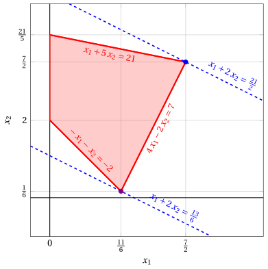
Exercise 11.13: Revised simplex algorithm (B1)

Consider the following LP problem in canonical maximization form with \(n=2\) variables and \(m=2\) constraints:

\[ \begin{array}{rrrrrr} {\max} & {25}\, {x_1} & {+} & {16}\, {x_2} \\[2ex] \text{subject to} & {50}\, {x_1} & {+} & {31}\, {x_2} & {\le} & {250} \\[2ex] & {-3}\, {x_1} & {+} & {2}\, {x_2} & {\le} & {4} \\[2ex] & {x_1,} & & {x_2} & {\ge} & {0} \end{array} \]

By introducing the slack variables, we get the following LP problem in standard maximization form with \(n+m=4\) variables and \(m=2\) constraints:

\[ \begin{array}{rrrrrrrrrr} {\max} & {25}\, {x_1} & {+} & {16}\, {x_2} \\[2ex] \text{subject to} & {50}\, {x_1} & {+} & {31}\, {x_2} & {+} & {x_3} & & & {=} & {250} \\[2ex] & {-3}\, {x_1} & {+} & {2}\, {x_2} & & & {+} & {x_4} & {=} & {4} \\[2ex] & {x_1,} & & {x_2,} & & {x_3,} & & {x_4} & {\ge} & {0} \end{array} \]

Questions

• Execute the revised simplex algorithm to find an optimal solution of this LP problem using Bland's rule to select the pivot column and the pivot row.

Solution

We have:

\[ {\boldsymbol A}= \begin{pmatrix} 50 & 31 & 1 & 0\\ -3 & 2 & 0 & 1 \end{pmatrix} \quad {\boldsymbol b}= \begin{pmatrix} 250\\ 4 \end{pmatrix} \quad {\boldsymbol c}= \begin{pmatrix} 25\\ 16\\ 0\\ 0 \end{pmatrix} \quad {\boldsymbol x}= \begin{pmatrix} x_1 \\ x_2 \\ x_3 \\ x_4 \end{pmatrix} \]

• Initialization

  Since it is an LP problem in standard form obtained from an LP problem in canonical form with \(~{\boldsymbol b} \ge 0\) by adding the slack variables, the partition \(\pazocal{B}=\{3,4\}\) and \(\pazocal{N}=\{1,2\}\) is associated with the following basic feasible solution:

  \[ \begin{pmatrix} x_3 \\ x_4 \end{pmatrix} = \begin{pmatrix} 250\\ 4 \end{pmatrix} \text{ and } \begin{pmatrix} x_1 \\ x_2 \end{pmatrix} = \begin{pmatrix} 0\\ 0 \end{pmatrix} \]

• Iteration 1

  With \(\pazocal{B}= \{3,~~4\}\) and \(\pazocal{N}= \{1,~~2\}\), we have:

  \[ {\boldsymbol x}_{\pazocal{B}}= \begin{pmatrix} x_3 \\ x_4 \end{pmatrix} ~~ {\boldsymbol A}_{\pazocal{B}}= \begin{pmatrix} 1 & 0\\ 0 & 1 \end{pmatrix} ~~ {\boldsymbol c}_{\pazocal{B}}= \begin{pmatrix} 0\\ 0 \end{pmatrix} ~~ {{ \bar{\boldsymbol b}}}= \begin{pmatrix} 250\\ 4 \end{pmatrix} \]
  \[ {\boldsymbol x}_{\pazocal{N}}= \begin{pmatrix} x_1 \\ x_2 \end{pmatrix} ~~ {\boldsymbol A}_{\pazocal{N}}= \begin{pmatrix} 50 & 31\\ -3 & 2 \end{pmatrix} ~~ {\boldsymbol c}_{\pazocal{N}}= \begin{pmatrix} 25\\ 16 \end{pmatrix} \]

  Optimality check

  We solve \({\boldsymbol \pi} \; {\boldsymbol A}_{\pazocal{B}} = {\boldsymbol c}'_{\pazocal{B}}\) to compute \({\boldsymbol \pi} = {{{\boldsymbol c}'_{\pazocal{B}} \; {\boldsymbol A}_{\pazocal{B}}^{-1}}}\), first system of linear equations:

  \[\begin{equation*} \begin{cases} \begin{array}{rrrrr} {\pi_3} & & & {=} & {0} \\[2ex] & & {\pi_4} & {=} & {0} \end{array} \end{cases} \qquad {\boldsymbol \pi}= \begin{pmatrix} 0 & 0\\ \end{pmatrix} \end{equation*}\]

  We compute the basic feasible solution value \({\bar{z}} = {\boldsymbol \pi} \; {\boldsymbol b} = \begin{pmatrix} 0 & 0\\ \end{pmatrix} \begin{pmatrix} 250\\ 4 \end{pmatrix} = 0\)

  We compute the reduced costs \({{ \bar{\boldsymbol c}}'} = {{\boldsymbol c}'_{\pazocal{N}} - {\boldsymbol \pi} \; {\boldsymbol A}_{\pazocal{N}}}\):

  \[ {{ \bar{\boldsymbol c}}'} = \begin{pmatrix} 25 & 16\\ \end{pmatrix} - \begin{pmatrix} 0 & 0\\ \end{pmatrix} \begin{pmatrix} 50 & 31\\ -3 & 2 \end{pmatrix} = \underbrace{ \begin{pmatrix} 25 & 16\\ \end{pmatrix} }_{{c_{1}~~~c_{2}}} - \underbrace{ \begin{pmatrix} 0 & 0\\ \end{pmatrix} }_{{\boldsymbol \pi}\;{\boldsymbol A}_{1} ~~{\boldsymbol \pi}\;{\boldsymbol A}_{2}} = \underbrace{ \begin{pmatrix} 25 & 16\\ \end{pmatrix} }_{{\bar{c}_{1}~~~\bar{c}_{2}}} \]

  Not all reduced costs are non-positive then we perform a pivoting operation.

  Pivoting operation

  Since \({c}_{1} > {\boldsymbol \pi} \;{\boldsymbol A}_{1}\), \(x_1\) is the pivot column and we have \({\boldsymbol A}_{1} = \begin{pmatrix} 50\\ -3 \end{pmatrix}\)

  We solve \({\boldsymbol A}_{\pazocal{B}} \; {\boldsymbol d} = {\boldsymbol A}_{1}\) to compute \({\boldsymbol d}={ {\boldsymbol A}_{\pazocal{B}}^{-1}} {\boldsymbol A}_{1}\), second system of linear equations:

  \[\begin{equation*} \begin{cases} \begin{array}{rrrrr} {d_3} & & & {=} & {50} \\[2ex] & & {d_4} & {=} & {-3} \end{array} \end{cases} \qquad {\boldsymbol d}= \begin{pmatrix} 50\\ -3 \end{pmatrix} \end{equation*}\]

  We have to find the largest \(t\) such that \({{ \bar{\boldsymbol b}}} - t \; {{\boldsymbol d}} \ge 0\):

  \[ \begin{cases} \underbrace{250 -t \cdot 50\ge 0}_{x_3 \ge 0} \\[2ex] \underbrace{4 -t \cdot \left( -3\right)\ge 0}_{x_4 \ge 0} \end{cases} \qquad \begin{cases} t\le 5 \\[2ex] t\ge -\dfrac{4}{3} \end{cases} \text{ then } t_{m}=5 \]

  Accordingly the value of the pivot column becomes \(t_{m}\), i.e., \(x_1=5\). The value of \(x_3\) becomes zero and \(x_3\) is the pivot row. The other basic variables take values \({ \bar{\boldsymbol b}} - t_{m} \; {\boldsymbol d}\), then we have:

  \[ x_4 = 4 - 5 \cdot \left( -3\right) = 19 \]

• Iteration 2

  With \(\pazocal{B}= \{1,~~4\}\) and \(\pazocal{N}= \{2,~~3\}\), we have:

  \[ {\boldsymbol x}_{\pazocal{B}}= \begin{pmatrix} x_1 \\ x_4 \end{pmatrix} ~~ {\boldsymbol A}_{\pazocal{B}}= \begin{pmatrix} 50 & 0\\ -3 & 1 \end{pmatrix} ~~ {\boldsymbol c}_{\pazocal{B}}= \begin{pmatrix} 25\\ 0 \end{pmatrix} ~~ {{ \bar{\boldsymbol b}}}= \begin{pmatrix} 5\\ 19 \end{pmatrix} \]
  \[ {\boldsymbol x}_{\pazocal{N}}= \begin{pmatrix} x_2 \\ x_3 \end{pmatrix} ~~ {\boldsymbol A}_{\pazocal{N}}= \begin{pmatrix} 31 & 1\\ 2 & 0 \end{pmatrix} ~~ {\boldsymbol c}_{\pazocal{N}}= \begin{pmatrix} 16\\ 0 \end{pmatrix} \]

  Optimality check

  We solve \({\boldsymbol \pi} \; {\boldsymbol A}_{\pazocal{B}} = {\boldsymbol c}'_{\pazocal{B}}\) to compute \({\boldsymbol \pi} = {{{\boldsymbol c}'_{\pazocal{B}} \; {\boldsymbol A}_{\pazocal{B}}^{-1}}}\), first system of linear equations:

  \[\begin{equation*} \begin{cases} \begin{array}{rrrrr} {50}\, {\pi_1} & {-} & {3}\, {\pi_4} & {=} & {25} \\[2ex] & & {\pi_4} & {=} & {0} \end{array} \end{cases} \qquad {\boldsymbol \pi}= \begin{pmatrix} \dfrac{1}{2} & 0\\ \end{pmatrix} \end{equation*}\]

  We compute the basic feasible solution value \({\bar{z}} = {\boldsymbol \pi} \; {\boldsymbol b} = \begin{pmatrix} \dfrac{1}{2} & 0\\ \end{pmatrix} \begin{pmatrix} 250\\ 4 \end{pmatrix} = 125\)

  We compute the reduced costs \({{ \bar{\boldsymbol c}}'} = {{\boldsymbol c}'_{\pazocal{N}} - {\boldsymbol \pi} \; {\boldsymbol A}_{\pazocal{N}}}\):

  \[ {{ \bar{\boldsymbol c}}'} = \begin{pmatrix} 16 & 0\\ \end{pmatrix} - \begin{pmatrix} \dfrac{1}{2} & 0\\ \end{pmatrix} \begin{pmatrix} 31 & 1\\ 2 & 0 \end{pmatrix} = \underbrace{ \begin{pmatrix} 16 & 0\\ \end{pmatrix} }_{{c_{2}~~~c_{3}}} - \underbrace{ \begin{pmatrix} \dfrac{31}{2} & \dfrac{1}{2}\\ \end{pmatrix} }_{{\boldsymbol \pi}\;{\boldsymbol A}_{2} ~~{\boldsymbol \pi}\;{\boldsymbol A}_{3}} = \underbrace{ \begin{pmatrix} \dfrac{1}{2} & -\dfrac{1}{2}\\ \end{pmatrix} }_{{\bar{c}_{2}~~~\bar{c}_{3}}} \]

  Not all reduced costs are non-positive then we perform a pivoting operation.

  Pivoting operation

  Since \({c}_{2} > {\boldsymbol \pi} \;{\boldsymbol A}_{2}\), \(x_2\) is the pivot column and we have \({\boldsymbol A}_{2} = \begin{pmatrix} 31\\ 2 \end{pmatrix}\)

  We solve \({\boldsymbol A}_{\pazocal{B}} \; {\boldsymbol d} = {\boldsymbol A}_{2}\) to compute \({\boldsymbol d}={ {\boldsymbol A}_{\pazocal{B}}^{-1}} {\boldsymbol A}_{2}\), second system of linear equations:

  \[\begin{equation*} \begin{cases} \begin{array}{rrrrr} {50}\, {d_1} & & & {=} & {31} \\[2ex] {-3}\, {d_1} & {+} & {d_4} & {=} & {2} \end{array} \end{cases} \qquad {\boldsymbol d}= \begin{pmatrix} \dfrac{31}{50}\\[2ex] \dfrac{193}{50} \end{pmatrix} \end{equation*}\]

  We have to find the largest \(t\) such that \({{ \bar{\boldsymbol b}}} - t \; {{\boldsymbol d}} \ge 0\):

  \[ \begin{cases} \underbrace{5 -t \cdot \dfrac{31}{50}\ge 0}_{x_1 \ge 0} \\[2ex] \underbrace{19 -t \cdot \dfrac{193}{50}\ge 0}_{x_4 \ge 0} \end{cases} \qquad \begin{cases} t\le \dfrac{250}{31} \\[2ex] t\le \dfrac{950}{193} \end{cases} \text{ then } t_{m}=\dfrac{950}{193} \]

  Accordingly the value of the pivot column becomes \(t_{m}\), i.e., \(x_2=\dfrac{950}{193}\). The value of \(x_4\) becomes zero and \(x_4\) is the pivot row. The other basic variables take values \({ \bar{\boldsymbol b}} - t_{m} \; {\boldsymbol d}\), then we have:

  \[ x_1 = 5 - \dfrac{950}{193} \cdot \dfrac{31}{50} = \dfrac{376}{193} \]

• Iteration 3

  With \(\pazocal{B}= \{1,~~2\}\) and \(\pazocal{N}= \{3,~~4\}\), we have:

  \[ {\boldsymbol x}_{\pazocal{B}}= \begin{pmatrix} x_1 \\ x_2 \end{pmatrix} ~~ {\boldsymbol A}_{\pazocal{B}}= \begin{pmatrix} 50 & 31\\ -3 & 2 \end{pmatrix} ~~ {\boldsymbol c}_{\pazocal{B}}= \begin{pmatrix} 25\\ 16 \end{pmatrix} ~~ {{ \bar{\boldsymbol b}}}= \begin{pmatrix} \dfrac{376}{193}\\[2ex] \dfrac{950}{193} \end{pmatrix} \]
  \[ {\boldsymbol x}_{\pazocal{N}}= \begin{pmatrix} x_3 \\ x_4 \end{pmatrix} ~~ {\boldsymbol A}_{\pazocal{N}}= \begin{pmatrix} 1 & 0\\ 0 & 1 \end{pmatrix} ~~ {\boldsymbol c}_{\pazocal{N}}= \begin{pmatrix} 0\\ 0 \end{pmatrix} \]

  Optimality check

  We solve \({\boldsymbol \pi} \; {\boldsymbol A}_{\pazocal{B}} = {\boldsymbol c}'_{\pazocal{B}}\) to compute \({\boldsymbol \pi} = {{{\boldsymbol c}'_{\pazocal{B}} \; {\boldsymbol A}_{\pazocal{B}}^{-1}}}\), first system of linear equations:

  \[\begin{equation*} \begin{cases} \begin{array}{rrrrr} {50}\, {\pi_1} & {-} & {3}\, {\pi_2} & {=} & {25} \\[2ex] {31}\, {\pi_1} & {+} & {2}\, {\pi_2} & {=} & {16} \end{array} \end{cases} \qquad {\boldsymbol \pi}= \begin{pmatrix} \dfrac{98}{193} & \dfrac{25}{193}\\ \end{pmatrix} \end{equation*}\]

  We compute the basic feasible solution value \({\bar{z}} = {\boldsymbol \pi} \; {\boldsymbol b} = \begin{pmatrix} \dfrac{98}{193} & \dfrac{25}{193}\\ \end{pmatrix} \begin{pmatrix} 250\\ 4 \end{pmatrix} = \dfrac{24600}{193}\)

  We compute the reduced costs \({{ \bar{\boldsymbol c}}'} = {{\boldsymbol c}'_{\pazocal{N}} - {\boldsymbol \pi} \; {\boldsymbol A}_{\pazocal{N}}}\):

  \[ {{ \bar{\boldsymbol c}}'} = \begin{pmatrix} 0 & 0\\ \end{pmatrix} - \begin{pmatrix} \dfrac{98}{193} & \dfrac{25}{193}\\ \end{pmatrix} \begin{pmatrix} 1 & 0\\ 0 & 1 \end{pmatrix} = \underbrace{ \begin{pmatrix} 0 & 0\\ \end{pmatrix} }_{{c_{3}~~~c_{4}}} - \underbrace{ \begin{pmatrix} \dfrac{98}{193} & \dfrac{25}{193}\\ \end{pmatrix} }_{{\boldsymbol \pi}\;{\boldsymbol A}_{3} ~~{\boldsymbol \pi}\;{\boldsymbol A}_{4}} = \underbrace{ \begin{pmatrix} -\dfrac{98}{193} & -\dfrac{25}{193}\\ \end{pmatrix} }_{{\bar{c}_{3}~~~\bar{c}_{4}}} \]

  All reduced costs are non-positive, then the basic feasible solution

  \[ {\boldsymbol x}_{\pazocal{B}}= \begin{pmatrix} x_1 \\ x_2 \end{pmatrix}=\begin{pmatrix} \dfrac{376}{193}\\[2ex] \dfrac{950}{193} \end{pmatrix} \text{ and } {\boldsymbol x}_{\pazocal{N}}= \begin{pmatrix} x_3 \\ x_4 \end{pmatrix}=\begin{pmatrix} 0\\ 0 \end{pmatrix} \]

  is an optimal solution of the LP problem and \({\bar{z}} = \dfrac{24600}{193}\) is the optimal solution value.

Graphical solution:

The feasible region of the LP problem (in canonical form) is the polyhedron shaded in red:

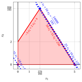
An optimal solution \({ \tilde{\boldsymbol x}}(\,LP\,)\) is:

\[ \tilde{x}_1=\dfrac{376}{193},~~ \tilde{x}_2=\dfrac{950}{193} \]

the optimal value \(z(\, LP\,)\) is \(\dfrac{24600}{193}.\)

In violet the first and the second vertex explored by the previous execution of the revised simplex algorithm (before reaching the optimal one depicted in blue).

In dashed blue, the contour lines of the objective function associated with the values taken in the three vertices.

Problems with three variables

Exercise 11.14: Revised simplex algorithm (P41)

Consider the following LP problem in canonical maximization form with \(n=3\) variables and \(m=4\) constraints:

\[ \begin{array}{rrrrrrrr} {\max} & {2}\, {x_1} & {+} & {x_2} & {+} & {3}\, {x_3} \\[2ex] \text{subject to} & {x_1} & {+} & {x_2} & {+} & {x_3} & {\le} & {4} \\[2ex] & & & {x_2} & & & {\le} & {2} \\[2ex] & & & & & {x_3} & {\le} & {3} \\[2ex] & {3}\, {x_1} & & & {+} & {x_3} & {\le} & {6} \\[2ex] & {x_1,} & & {x_2,} & & {x_3} & {\ge} & {0} \end{array} \]

By introducing the slack variables, we get the following LP problem in standard maximization form with \(n+m=7\) variables and \(m=4\) constraints:

\[ \begin{array}{rrcrcrcrcrcrcrcr} {\max} & {2}\, {x_1} & {+} & {x_2} & {+} & {3}\, {x_3} \\[2ex] \text{subject to} & {x_1} & {+} & {x_2} & {+} & {x_3} & {+} & {x_4} & & & & & & & {=} & {4} \\[2ex] & & & {x_2} & & & & & {+} & {x_5} & & & & & {=} & {2} \\[2ex] & & & & & {x_3} & & & & & {+} & {x_6} & & & {=} & {3} \\[2ex] & {3}\, {x_1} & & & {+} & {x_3} & & & & & & & {+} & {x_7} & {=} & {6} \\[2ex] & {x_1,} & & {x_2,} & & {x_3,} & & {x_4,} & & {x_5,} & & {x_6,} & & {x_7} & {\ge} & {0} \end{array} \]

Questions

• Execute the revised simplex algorithm to find an optimal solution of this LP problem using Bland's rule to select the pivot column and the pivot row.

Solution

We have:

\[ {\boldsymbol A}= \begin{pmatrix} 1 & 1 & 1 & 1 & 0 & 0 & 0\\ 0 & 1 & 0 & 0 & 1 & 0 & 0\\ 0 & 0 & 1 & 0 & 0 & 1 & 0\\ 3 & 0 & 1 & 0 & 0 & 0 & 1 \end{pmatrix} \quad {\boldsymbol b}= \begin{pmatrix} 4\\ 2\\ 3\\ 6 \end{pmatrix} \quad {\boldsymbol c}= \begin{pmatrix} 2\\ 1\\ 3\\ 0\\ 0\\ 0\\ 0 \end{pmatrix} \quad {\boldsymbol x}= \begin{pmatrix} x_1 \\ x_2 \\ x_3 \\ x_4 \\ x_5 \\ x_6 \\ x_7 \end{pmatrix} \]

• Initialization

  Since it is an LP problem in standard form obtained from an LP problem in canonical form with \(~{\boldsymbol b} \ge 0\) by adding the slack variables, the partition \(\pazocal{B}=\{4,5,6,7\}\) and \(\pazocal{N}=\{1,2,3\}\) is associated with the following basic feasible solution:

  \[ \begin{pmatrix} x_4 \\ x_5 \\ x_6 \\ x_7 \end{pmatrix} = \begin{pmatrix} 4\\ 2\\ 3\\ 6 \end{pmatrix} \text{ and } \begin{pmatrix} x_1 \\ x_2 \\ x_3 \end{pmatrix} = \begin{pmatrix} 0\\ 0\\ 0 \end{pmatrix} \]

• Iteration 1

  With \(\pazocal{B}= \{4,~~5,~~6,~~7\}\) and \(\pazocal{N}= \{1,~~2,~~3\}\), we have:

  \[ {\boldsymbol x}_{\pazocal{B}}= \begin{pmatrix} x_4 \\ x_5 \\ x_6 \\ x_7 \end{pmatrix} ~~ {\boldsymbol A}_{\pazocal{B}}= \begin{pmatrix} 1 & 0 & 0 & 0\\ 0 & 1 & 0 & 0\\ 0 & 0 & 1 & 0\\ 0 & 0 & 0 & 1 \end{pmatrix} ~~ {\boldsymbol c}_{\pazocal{B}}= \begin{pmatrix} 0\\ 0\\ 0\\ 0 \end{pmatrix} ~~ {{ \bar{\boldsymbol b}}}= \begin{pmatrix} 4\\ 2\\ 3\\ 6 \end{pmatrix} \]
  \[ {\boldsymbol x}_{\pazocal{N}}= \begin{pmatrix} x_1 \\ x_2 \\ x_3 \end{pmatrix} ~~ {\boldsymbol A}_{\pazocal{N}}= \begin{pmatrix} 1 & 1 & 1\\ 0 & 1 & 0\\ 0 & 0 & 1\\ 3 & 0 & 1 \end{pmatrix} ~~ {\boldsymbol c}_{\pazocal{N}}= \begin{pmatrix} 2\\ 1\\ 3 \end{pmatrix} \]

  Optimality check

  We solve \({\boldsymbol \pi} \; {\boldsymbol A}_{\pazocal{B}} = {\boldsymbol c}'_{\pazocal{B}}\) to compute \({\boldsymbol \pi} = {{{\boldsymbol c}'_{\pazocal{B}} \; {\boldsymbol A}_{\pazocal{B}}^{-1}}}\), first system of linear equations:

  \[\begin{equation*} \begin{cases} \begin{array}{rrrrrrrrr} {\pi_4} & & & & & & & {=} & {0} \\[2ex] & & {\pi_5} & & & & & {=} & {0} \\[2ex] & & & & {\pi_6} & & & {=} & {0} \\[2ex] & & & & & & {\pi_7} & {=} & {0} \end{array} \end{cases} \qquad {\boldsymbol \pi}= \begin{pmatrix} 0 & 0 & 0 & 0\\ \end{pmatrix} \end{equation*}\]

  We compute the basic feasible solution value \({\bar{z}} = {\boldsymbol \pi} \; {\boldsymbol b} = \begin{pmatrix} 0 & 0 & 0 & 0\\ \end{pmatrix} \begin{pmatrix} 4\\ 2\\ 3\\ 6 \end{pmatrix} = 0\)

  We compute the reduced costs \({{ \bar{\boldsymbol c}}'} = {{\boldsymbol c}'_{\pazocal{N}} - {\boldsymbol \pi} \; {\boldsymbol A}_{\pazocal{N}}}\):

  \[ \begin{aligned} {{ \bar{\boldsymbol c}}'} &= \begin{pmatrix} 2 & 1 & 3\\ \end{pmatrix} - \begin{pmatrix} 0 & 0 & 0 & 0\\ \end{pmatrix} \begin{pmatrix} 1 & 1 & 1\\ 0 & 1 & 0\\ 0 & 0 & 1\\ 3 & 0 & 1 \end{pmatrix} \\[1ex] &= \underbrace{ \begin{pmatrix} 2 & 1 & 3\\ \end{pmatrix} }_{{c_{1}~~~c_{2}~~~c_{3}}} - \underbrace{ \begin{pmatrix} 0 & 0 & 0\\ \end{pmatrix} }_{{\boldsymbol \pi}\;{\boldsymbol A}_{1} ~~{\boldsymbol \pi}\;{\boldsymbol A}_{2} ~~{\boldsymbol \pi}\;{\boldsymbol A}_{3}} = \underbrace{ \begin{pmatrix} 2 & 1 & 3\\ \end{pmatrix} }_{{\bar{c}_{1}~~~\bar{c}_{2}~~~\bar{c}_{3}}} \end{aligned} \]

  Not all reduced costs are non-positive then we perform a pivoting operation.

  Pivoting operation

  Since \({c}_{1} > {\boldsymbol \pi} \;{\boldsymbol A}_{1}\), \(x_1\) is the pivot column and we have \({\boldsymbol A}_{1} = \begin{pmatrix} 1\\ 0\\ 0\\ 3 \end{pmatrix}\)

  We solve \({\boldsymbol A}_{\pazocal{B}} \; {\boldsymbol d} = {\boldsymbol A}_{1}\) to compute \({\boldsymbol d}={ {\boldsymbol A}_{\pazocal{B}}^{-1}} {\boldsymbol A}_{1}\), second system of linear equations:

  \[\begin{equation*} \begin{cases} \begin{array}{rrrrrrrrr} {d_4} & & & & & & & {=} & {1} \\[2ex] & & {d_5} & & & & & {=} & {0} \\[2ex] & & & & {d_6} & & & {=} & {0} \\[2ex] & & & & & & {d_7} & {=} & {3} \end{array} \end{cases} \qquad {\boldsymbol d}= \begin{pmatrix} 1\\ 0\\ 0\\ 3 \end{pmatrix} \end{equation*}\]

  We have to find the largest \(t\) such that \({{ \bar{\boldsymbol b}}} - t \; {{\boldsymbol d}} \ge 0\):

  \[ \begin{cases} \underbrace{4 -t \cdot 1\ge 0}_{x_4 \ge 0} \\[2ex] \underbrace{6 -t \cdot 3\ge 0}_{x_7 \ge 0} \end{cases} \qquad \begin{cases} t\le 4 \\[2ex] t\le 2 \end{cases} \text{ then } t_{m}=2 \]

  Accordingly the value of the pivot column becomes \(t_{m}\), i.e., \(x_1=2\). The value of \(x_7\) becomes zero and \(x_7\) is the pivot row. The other basic variables take values \({ \bar{\boldsymbol b}} - t_{m} \; {\boldsymbol d}\), then we have:

  \[ \begin{aligned} x_4 &= 4 - 2 \cdot 1 = 2 \\[2ex] x_5 &= 2 - 2 \cdot 0 = 2 \\[2ex] x_6 &= 3 - 2 \cdot 0 = 3 \end{aligned} \]

• Iteration 2

  With \(\pazocal{B}= \{1,~~4,~~5,~~6\}\) and \(\pazocal{N}= \{2,~~3,~~7\}\), we have:

  \[ {\boldsymbol x}_{\pazocal{B}}= \begin{pmatrix} x_1 \\ x_4 \\ x_5 \\ x_6 \end{pmatrix} ~~ {\boldsymbol A}_{\pazocal{B}}= \begin{pmatrix} 1 & 1 & 0 & 0\\ 0 & 0 & 1 & 0\\ 0 & 0 & 0 & 1\\ 3 & 0 & 0 & 0 \end{pmatrix} ~~ {\boldsymbol c}_{\pazocal{B}}= \begin{pmatrix} 2\\ 0\\ 0\\ 0 \end{pmatrix} ~~ {{ \bar{\boldsymbol b}}}= \begin{pmatrix} 2\\ 2\\ 2\\ 3 \end{pmatrix} \]
  \[ {\boldsymbol x}_{\pazocal{N}}= \begin{pmatrix} x_2 \\ x_3 \\ x_7 \end{pmatrix} ~~ {\boldsymbol A}_{\pazocal{N}}= \begin{pmatrix} 1 & 1 & 0\\ 1 & 0 & 0\\ 0 & 1 & 0\\ 0 & 1 & 1 \end{pmatrix} ~~ {\boldsymbol c}_{\pazocal{N}}= \begin{pmatrix} 1\\ 3\\ 0 \end{pmatrix} \]

  Optimality check

  We solve \({\boldsymbol \pi} \; {\boldsymbol A}_{\pazocal{B}} = {\boldsymbol c}'_{\pazocal{B}}\) to compute \({\boldsymbol \pi} = {{{\boldsymbol c}'_{\pazocal{B}} \; {\boldsymbol A}_{\pazocal{B}}^{-1}}}\), first system of linear equations:

  \[\begin{equation*} \begin{cases} \begin{array}{rrrrrrrrr} {\pi_1} & & & & & {+} & {3}\, {\pi_6} & {=} & {2} \\[2ex] {\pi_1} & & & & & & & {=} & {0} \\[2ex] & & {\pi_4} & & & & & {=} & {0} \\[2ex] & & & & {\pi_5} & & & {=} & {0} \end{array} \end{cases} \qquad {\boldsymbol \pi}= \begin{pmatrix} 0 & 0 & 0 & \dfrac{2}{3}\\ \end{pmatrix} \end{equation*}\]

  We compute the basic feasible solution value \({\bar{z}} = {\boldsymbol \pi} \; {\boldsymbol b} = \begin{pmatrix} 0 & 0 & 0 & \dfrac{2}{3}\\ \end{pmatrix} \begin{pmatrix} 4\\ 2\\ 3\\ 6 \end{pmatrix} = 4\)

  We compute the reduced costs \({{ \bar{\boldsymbol c}}'} = {{\boldsymbol c}'_{\pazocal{N}} - {\boldsymbol \pi} \; {\boldsymbol A}_{\pazocal{N}}}\):

  \[ \begin{aligned} {{ \bar{\boldsymbol c}}'} &= \begin{pmatrix} 1 & 3 & 0\\ \end{pmatrix} - \begin{pmatrix} 0 & 0 & 0 & \dfrac{2}{3}\\ \end{pmatrix} \begin{pmatrix} 1 & 1 & 0\\ 1 & 0 & 0\\ 0 & 1 & 0\\ 0 & 1 & 1 \end{pmatrix} \\[1ex] &= \underbrace{ \begin{pmatrix} 1 & 3 & 0\\ \end{pmatrix} }_{{c_{2}~~~c_{3}~~~c_{7}}} - \underbrace{ \begin{pmatrix} 0 & \dfrac{2}{3} & \dfrac{2}{3}\\ \end{pmatrix} }_{{\boldsymbol \pi}\;{\boldsymbol A}_{2} ~~{\boldsymbol \pi}\;{\boldsymbol A}_{3} ~~{\boldsymbol \pi}\;{\boldsymbol A}_{7}} = \underbrace{ \begin{pmatrix} 1 & \dfrac{7}{3} & -\dfrac{2}{3}\\ \end{pmatrix} }_{{\bar{c}_{2}~~~\bar{c}_{3}~~~\bar{c}_{7}}} \end{aligned} \]

  Not all reduced costs are non-positive then we perform a pivoting operation.

  Pivoting operation

  Since \({c}_{2} > {\boldsymbol \pi} \;{\boldsymbol A}_{2}\), \(x_2\) is the pivot column and we have \({\boldsymbol A}_{2} = \begin{pmatrix} 1\\ 1\\ 0\\ 0 \end{pmatrix}\)

  We solve \({\boldsymbol A}_{\pazocal{B}} \; {\boldsymbol d} = {\boldsymbol A}_{2}\) to compute \({\boldsymbol d}={ {\boldsymbol A}_{\pazocal{B}}^{-1}} {\boldsymbol A}_{2}\), second system of linear equations:

  \[\begin{equation*} \begin{cases} \begin{array}{rrrrrrrrr} {d_1} & {+} & {d_4} & & & & & {=} & {1} \\[2ex] & & & & {d_5} & & & {=} & {1} \\[2ex] & & & & & & {d_6} & {=} & {0} \\[2ex] {3}\, {d_1} & & & & & & & {=} & {0} \end{array} \end{cases} \qquad {\boldsymbol d}= \begin{pmatrix} 0\\ 1\\ 1\\ 0 \end{pmatrix} \end{equation*}\]

  We have to find the largest \(t\) such that \({{ \bar{\boldsymbol b}}} - t \; {{\boldsymbol d}} \ge 0\):

  \[ \begin{cases} \underbrace{2 -t \cdot 1\ge 0}_{x_4 \ge 0} \\[2ex] \underbrace{2 -t \cdot 1\ge 0}_{x_5 \ge 0} \end{cases} \qquad \begin{cases} t\le 2 \\[2ex] t\le 2 \end{cases} \text{ then } t_{m}=2 \]

  Accordingly the value of the pivot column becomes \(t_{m}\), i.e., \(x_2=2\). The value of \(x_4\) becomes zero and \(x_4\) is the pivot row. The other basic variables take values \({ \bar{\boldsymbol b}} - t_{m} \; {\boldsymbol d}\), then we have:

  \[ \begin{aligned} x_1 &= 2 - 2 \cdot 0 = 2 \\[2ex] x_5 &= 2 - 2 \cdot 1 = 0 \\[2ex] x_6 &= 3 - 2 \cdot 0 = 3 \end{aligned} \]

• Iteration 3

  With \(\pazocal{B}= \{1,~~2,~~5,~~6\}\) and \(\pazocal{N}= \{3,~~4,~~7\}\), we have:

  \[ {\boldsymbol x}_{\pazocal{B}}= \begin{pmatrix} x_1 \\ x_2 \\ x_5 \\ x_6 \end{pmatrix} ~~ {\boldsymbol A}_{\pazocal{B}}= \begin{pmatrix} 1 & 1 & 0 & 0\\ 0 & 1 & 1 & 0\\ 0 & 0 & 0 & 1\\ 3 & 0 & 0 & 0 \end{pmatrix} ~~ {\boldsymbol c}_{\pazocal{B}}= \begin{pmatrix} 2\\ 1\\ 0\\ 0 \end{pmatrix} ~~ {{ \bar{\boldsymbol b}}}= \begin{pmatrix} 2\\ 2\\ 0\\ 3 \end{pmatrix} \]
  \[ {\boldsymbol x}_{\pazocal{N}}= \begin{pmatrix} x_3 \\ x_4 \\ x_7 \end{pmatrix} ~~ {\boldsymbol A}_{\pazocal{N}}= \begin{pmatrix} 1 & 1 & 0\\ 0 & 0 & 0\\ 1 & 0 & 0\\ 1 & 0 & 1 \end{pmatrix} ~~ {\boldsymbol c}_{\pazocal{N}}= \begin{pmatrix} 3\\ 0\\ 0 \end{pmatrix} \]

  Optimality check

  We solve \({\boldsymbol \pi} \; {\boldsymbol A}_{\pazocal{B}} = {\boldsymbol c}'_{\pazocal{B}}\) to compute \({\boldsymbol \pi} = {{{\boldsymbol c}'_{\pazocal{B}} \; {\boldsymbol A}_{\pazocal{B}}^{-1}}}\), first system of linear equations:

  \[\begin{equation*} \begin{cases} \begin{array}{rrrrrrrrr} {\pi_1} & & & & & {+} & {3}\, {\pi_6} & {=} & {2} \\[2ex] {\pi_1} & {+} & {\pi_2} & & & & & {=} & {1} \\[2ex] & & {\pi_2} & & & & & {=} & {0} \\[2ex] & & & & {\pi_5} & & & {=} & {0} \end{array} \end{cases} \qquad {\boldsymbol \pi}= \begin{pmatrix} 1 & 0 & 0 & \dfrac{1}{3}\\ \end{pmatrix} \end{equation*}\]

  We compute the basic feasible solution value \({\bar{z}} = {\boldsymbol \pi} \; {\boldsymbol b} = \begin{pmatrix} 1 & 0 & 0 & \dfrac{1}{3}\\ \end{pmatrix} \begin{pmatrix} 4\\ 2\\ 3\\ 6 \end{pmatrix} = 6\)

  We compute the reduced costs \({{ \bar{\boldsymbol c}}'} = {{\boldsymbol c}'_{\pazocal{N}} - {\boldsymbol \pi} \; {\boldsymbol A}_{\pazocal{N}}}\):

  \[ \begin{aligned} {{ \bar{\boldsymbol c}}'} &= \begin{pmatrix} 3 & 0 & 0\\ \end{pmatrix} - \begin{pmatrix} 1 & 0 & 0 & \dfrac{1}{3}\\ \end{pmatrix} \begin{pmatrix} 1 & 1 & 0\\ 0 & 0 & 0\\ 1 & 0 & 0\\ 1 & 0 & 1 \end{pmatrix} \\[1ex] &= \underbrace{ \begin{pmatrix} 3 & 0 & 0\\ \end{pmatrix} }_{{c_{3}~~~c_{4}~~~c_{7}}} - \underbrace{ \begin{pmatrix} \dfrac{4}{3} & 1 & \dfrac{1}{3}\\ \end{pmatrix} }_{{\boldsymbol \pi}\;{\boldsymbol A}_{3} ~~{\boldsymbol \pi}\;{\boldsymbol A}_{4} ~~{\boldsymbol \pi}\;{\boldsymbol A}_{7}} = \underbrace{ \begin{pmatrix} \dfrac{5}{3} & -1 & -\dfrac{1}{3}\\ \end{pmatrix} }_{{\bar{c}_{3}~~~\bar{c}_{4}~~~\bar{c}_{7}}} \end{aligned} \]

  Not all reduced costs are non-positive then we perform a pivoting operation.

  Pivoting operation

  Since \({c}_{3} > {\boldsymbol \pi} \;{\boldsymbol A}_{3}\), \(x_3\) is the pivot column and we have \({\boldsymbol A}_{3} = \begin{pmatrix} 1\\ 0\\ 1\\ 1 \end{pmatrix}\)

  We solve \({\boldsymbol A}_{\pazocal{B}} \; {\boldsymbol d} = {\boldsymbol A}_{3}\) to compute \({\boldsymbol d}={ {\boldsymbol A}_{\pazocal{B}}^{-1}} {\boldsymbol A}_{3}\), second system of linear equations:

  \[\begin{equation*} \begin{cases} \begin{array}{rrrrrrrrr} {d_1} & {+} & {d_2} & & & & & {=} & {1} \\[2ex] & & {d_2} & {+} & {d_5} & & & {=} & {0} \\[2ex] & & & & & & {d_6} & {=} & {1} \\[2ex] {3}\, {d_1} & & & & & & & {=} & {1} \end{array} \end{cases} \qquad {\boldsymbol d}= \begin{pmatrix} \dfrac{1}{3}\\[2ex] \dfrac{2}{3}\\[2ex] -\dfrac{2}{3}\\[2ex] 1 \end{pmatrix} \end{equation*}\]

  We have to find the largest \(t\) such that \({{ \bar{\boldsymbol b}}} - t \; {{\boldsymbol d}} \ge 0\):

  \[ \begin{cases} \underbrace{2 -t \cdot \dfrac{1}{3}\ge 0}_{x_1 \ge 0} \\[2ex] \underbrace{2 -t \cdot \dfrac{2}{3}\ge 0}_{x_2 \ge 0} \\[2ex] \underbrace{0 -t \cdot \left( -\dfrac{2}{3}\right)\ge 0}_{x_5 \ge 0} \\[2ex] \underbrace{3 -t \cdot 1\ge 0}_{x_6 \ge 0} \end{cases} \qquad \begin{cases} t\le 6 \\[2ex] t\le 3 \\[2ex] t\ge 0 \\[2ex] t\le 3 \end{cases} \text{ then } t_{m}=3 \]

  Accordingly the value of the pivot column becomes \(t_{m}\), i.e., \(x_3=3\). The value of \(x_2\) becomes zero and \(x_2\) is the pivot row. The other basic variables take values \({ \bar{\boldsymbol b}} - t_{m} \; {\boldsymbol d}\), then we have:

  \[ \begin{aligned} x_1 &= 2 - 3 \cdot \dfrac{1}{3} = 1 \\[2ex] x_5 &= 0 - 3 \cdot \left( -\dfrac{2}{3}\right) = 2 \\[2ex] x_6 &= 3 - 3 \cdot 1 = 0 \end{aligned} \]

• Iteration 4

  With \(\pazocal{B}= \{1,~~3,~~5,~~6\}\) and \(\pazocal{N}= \{2,~~4,~~7\}\), we have:

  \[ {\boldsymbol x}_{\pazocal{B}}= \begin{pmatrix} x_1 \\ x_3 \\ x_5 \\ x_6 \end{pmatrix} ~~ {\boldsymbol A}_{\pazocal{B}}= \begin{pmatrix} 1 & 1 & 0 & 0\\ 0 & 0 & 1 & 0\\ 0 & 1 & 0 & 1\\ 3 & 1 & 0 & 0 \end{pmatrix} ~~ {\boldsymbol c}_{\pazocal{B}}= \begin{pmatrix} 2\\ 3\\ 0\\ 0 \end{pmatrix} ~~ {{ \bar{\boldsymbol b}}}= \begin{pmatrix} 1\\ 3\\ 2\\ 0 \end{pmatrix} \]
  \[ {\boldsymbol x}_{\pazocal{N}}= \begin{pmatrix} x_2 \\ x_4 \\ x_7 \end{pmatrix} ~~ {\boldsymbol A}_{\pazocal{N}}= \begin{pmatrix} 1 & 1 & 0\\ 1 & 0 & 0\\ 0 & 0 & 0\\ 0 & 0 & 1 \end{pmatrix} ~~ {\boldsymbol c}_{\pazocal{N}}= \begin{pmatrix} 1\\ 0\\ 0 \end{pmatrix} \]

  Optimality check

  We solve \({\boldsymbol \pi} \; {\boldsymbol A}_{\pazocal{B}} = {\boldsymbol c}'_{\pazocal{B}}\) to compute \({\boldsymbol \pi} = {{{\boldsymbol c}'_{\pazocal{B}} \; {\boldsymbol A}_{\pazocal{B}}^{-1}}}\), first system of linear equations:

  \[\begin{equation*} \begin{cases} \begin{array}{rrrrrrrrr} {\pi_1} & & & & & {+} & {3}\, {\pi_6} & {=} & {2} \\[2ex] {\pi_1} & & & {+} & {\pi_5} & {+} & {\pi_6} & {=} & {3} \\[2ex] & & {\pi_3} & & & & & {=} & {0} \\[2ex] & & & & {\pi_5} & & & {=} & {0} \end{array} \end{cases} \qquad {\boldsymbol \pi}= \begin{pmatrix} \dfrac{7}{2} & 0 & 0 & -\dfrac{1}{2}\\ \end{pmatrix} \end{equation*}\]

  We compute the basic feasible solution value \({\bar{z}} = {\boldsymbol \pi} \; {\boldsymbol b} = \begin{pmatrix} \dfrac{7}{2} & 0 & 0 & -\dfrac{1}{2}\\ \end{pmatrix} \begin{pmatrix} 4\\ 2\\ 3\\ 6 \end{pmatrix} = 11\)

  We compute the reduced costs \({{ \bar{\boldsymbol c}}'} = {{\boldsymbol c}'_{\pazocal{N}} - {\boldsymbol \pi} \; {\boldsymbol A}_{\pazocal{N}}}\):

  \[ \begin{aligned} {{ \bar{\boldsymbol c}}'} &= \begin{pmatrix} 1 & 0 & 0\\ \end{pmatrix} - \begin{pmatrix} \dfrac{7}{2} & 0 & 0 & -\dfrac{1}{2}\\ \end{pmatrix} \begin{pmatrix} 1 & 1 & 0\\ 1 & 0 & 0\\ 0 & 0 & 0\\ 0 & 0 & 1 \end{pmatrix} \\[1ex] &= \underbrace{ \begin{pmatrix} 1 & 0 & 0\\ \end{pmatrix} }_{{c_{2}~~~c_{4}~~~c_{7}}} - \underbrace{ \begin{pmatrix} \dfrac{7}{2} & \dfrac{7}{2} & -\dfrac{1}{2}\\ \end{pmatrix} }_{{\boldsymbol \pi}\;{\boldsymbol A}_{2} ~~{\boldsymbol \pi}\;{\boldsymbol A}_{4} ~~{\boldsymbol \pi}\;{\boldsymbol A}_{7}} = \underbrace{ \begin{pmatrix} -\dfrac{5}{2} & -\dfrac{7}{2} & \dfrac{1}{2}\\ \end{pmatrix} }_{{\bar{c}_{2}~~~\bar{c}_{4}~~~\bar{c}_{7}}} \end{aligned} \]

  Not all reduced costs are non-positive then we perform a pivoting operation.

  Pivoting operation

  Since \({c}_{7} > {\boldsymbol \pi} \;{\boldsymbol A}_{7}\), \(x_7\) is the pivot column and we have \({\boldsymbol A}_{7} = \begin{pmatrix} 0\\ 0\\ 0\\ 1 \end{pmatrix}\)

  We solve \({\boldsymbol A}_{\pazocal{B}} \; {\boldsymbol d} = {\boldsymbol A}_{7}\) to compute \({\boldsymbol d}={ {\boldsymbol A}_{\pazocal{B}}^{-1}} {\boldsymbol A}_{7}\), second system of linear equations:

  \[\begin{equation*} \begin{cases} \begin{array}{rrrrrrrrr} {d_1} & {+} & {d_3} & & & & & {=} & {0} \\[2ex] & & & & {d_5} & & & {=} & {0} \\[2ex] & & {d_3} & & & {+} & {d_6} & {=} & {0} \\[2ex] {3}\, {d_1} & {+} & {d_3} & & & & & {=} & {1} \end{array} \end{cases} \qquad {\boldsymbol d}= \begin{pmatrix} \dfrac{1}{2}\\[2ex] -\dfrac{1}{2}\\[2ex] 0\\[2ex] \dfrac{1}{2} \end{pmatrix} \end{equation*}\]

  We have to find the largest \(t\) such that \({{ \bar{\boldsymbol b}}} - t \; {{\boldsymbol d}} \ge 0\):

  \[ \begin{cases} \underbrace{1 -t \cdot \dfrac{1}{2}\ge 0}_{x_1 \ge 0} \\[2ex] \underbrace{3 -t \cdot \left( -\dfrac{1}{2}\right)\ge 0}_{x_3 \ge 0} \\[2ex] \underbrace{0 -t \cdot \dfrac{1}{2}\ge 0}_{x_6 \ge 0} \end{cases} \qquad \begin{cases} t\le 2 \\[2ex] t\ge -6 \\[2ex] t\le 0 \end{cases} \text{ then } t_{m}=0 \]

  Accordingly the value of the pivot column becomes \(t_{m}\), i.e., \(x_7=0\). The value of \(x_6\) remains zero and \(x_6\) is the pivot row. The other basic variables take values \({ \bar{\boldsymbol b}} - t_{m} \; {\boldsymbol d}\), then we have:

  \[ \begin{aligned} x_1 &= 1 - 0 \cdot \dfrac{1}{2} = 1 \\[2ex] x_3 &= 3 - 0 \cdot \left( -\dfrac{1}{2}\right) = 3 \\[2ex] x_5 &= 2 - 0 \cdot 0 = 2 \end{aligned} \]

• Iteration 5

  With \(\pazocal{B}= \{1,~~3,~~5,~~7\}\) and \(\pazocal{N}= \{2,~~4,~~6\}\), we have:

  \[ {\boldsymbol x}_{\pazocal{B}}= \begin{pmatrix} x_1 \\ x_3 \\ x_5 \\ x_7 \end{pmatrix} ~~ {\boldsymbol A}_{\pazocal{B}}= \begin{pmatrix} 1 & 1 & 0 & 0\\ 0 & 0 & 1 & 0\\ 0 & 1 & 0 & 0\\ 3 & 1 & 0 & 1 \end{pmatrix} ~~ {\boldsymbol c}_{\pazocal{B}}= \begin{pmatrix} 2\\ 3\\ 0\\ 0 \end{pmatrix} ~~ {{ \bar{\boldsymbol b}}}= \begin{pmatrix} 1\\ 3\\ 2\\ 0 \end{pmatrix} \]
  \[ {\boldsymbol x}_{\pazocal{N}}= \begin{pmatrix} x_2 \\ x_4 \\ x_6 \end{pmatrix} ~~ {\boldsymbol A}_{\pazocal{N}}= \begin{pmatrix} 1 & 1 & 0\\ 1 & 0 & 0\\ 0 & 0 & 1\\ 0 & 0 & 0 \end{pmatrix} ~~ {\boldsymbol c}_{\pazocal{N}}= \begin{pmatrix} 1\\ 0\\ 0 \end{pmatrix} \]

  Optimality check

  We solve \({\boldsymbol \pi} \; {\boldsymbol A}_{\pazocal{B}} = {\boldsymbol c}'_{\pazocal{B}}\) to compute \({\boldsymbol \pi} = {{{\boldsymbol c}'_{\pazocal{B}} \; {\boldsymbol A}_{\pazocal{B}}^{-1}}}\), first system of linear equations:

  \[\begin{equation*} \begin{cases} \begin{array}{rrrrrrrrr} {\pi_1} & & & & & {+} & {3}\, {\pi_7} & {=} & {2} \\[2ex] {\pi_1} & & & {+} & {\pi_5} & {+} & {\pi_7} & {=} & {3} \\[2ex] & & {\pi_3} & & & & & {=} & {0} \\[2ex] & & & & & & {\pi_7} & {=} & {0} \end{array} \end{cases} \qquad {\boldsymbol \pi}= \begin{pmatrix} 2 & 0 & 1 & 0\\ \end{pmatrix} \end{equation*}\]

  We compute the basic feasible solution value \({\bar{z}} = {\boldsymbol \pi} \; {\boldsymbol b} = \begin{pmatrix} 2 & 0 & 1 & 0\\ \end{pmatrix} \begin{pmatrix} 4\\ 2\\ 3\\ 6 \end{pmatrix} = 11\)

  We compute the reduced costs \({{ \bar{\boldsymbol c}}'} = {{\boldsymbol c}'_{\pazocal{N}} - {\boldsymbol \pi} \; {\boldsymbol A}_{\pazocal{N}}}\):

  \[ \begin{aligned} {{ \bar{\boldsymbol c}}'} &= \begin{pmatrix} 1 & 0 & 0\\ \end{pmatrix} - \begin{pmatrix} 2 & 0 & 1 & 0\\ \end{pmatrix} \begin{pmatrix} 1 & 1 & 0\\ 1 & 0 & 0\\ 0 & 0 & 1\\ 0 & 0 & 0 \end{pmatrix} \\[1ex] &= \underbrace{ \begin{pmatrix} 1 & 0 & 0\\ \end{pmatrix} }_{{c_{2}~~~c_{4}~~~c_{6}}} - \underbrace{ \begin{pmatrix} 2 & 2 & 1\\ \end{pmatrix} }_{{\boldsymbol \pi}\;{\boldsymbol A}_{2} ~~{\boldsymbol \pi}\;{\boldsymbol A}_{4} ~~{\boldsymbol \pi}\;{\boldsymbol A}_{6}} = \underbrace{ \begin{pmatrix} -1 & -2 & -1\\ \end{pmatrix} }_{{\bar{c}_{2}~~~\bar{c}_{4}~~~\bar{c}_{6}}} \end{aligned} \]

  All reduced costs are non-positive, then the basic feasible solution

  \[ {\boldsymbol x}_{\pazocal{B}}= \begin{pmatrix} x_1 \\ x_3 \\ x_5 \\ x_7 \end{pmatrix}=\begin{pmatrix} 1\\ 3\\ 2\\ 0 \end{pmatrix} \text{ and } {\boldsymbol x}_{\pazocal{N}}= \begin{pmatrix} x_2 \\ x_4 \\ x_6 \end{pmatrix}=\begin{pmatrix} 0\\ 0\\ 0 \end{pmatrix} \]

  is an optimal solution of the LP problem and \({\bar{z}} = 11\) is the optimal solution value.

Graphical solution:

The feasible region of the LP problem (in canonical form) is the polyhedron shaded in red:

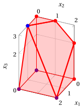
An optimal solution \({ \tilde{\boldsymbol x}}(\, LP \,)\) is:

\[ \tilde{x}_1=1,~~ \tilde{x}_2=0,~~ \tilde{x}_3=3 \]

the optimal value \(z(\, LP \,)\) is \(11.\)

In violet the first and the second vertex explored by the previous execution of the revised simplex algorithm (before reaching the optimal one depicted in blue).

Exercise 11.15: Revised simplex algorithm (P42)

Consider the following LP problem in canonical maximization form with \(n=3\) variables and \(m=3\) constraints:

\[ \begin{array}{rrrrrrrr} {\max} & {3}\, {x_1} & {+} & {2}\, {x_2} & {+} & {4}\, {x_3} \\[2ex] \text{subject to} & {x_1} & {+} & {x_2} & {+} & {2}\, {x_3} & {\le} & {4} \\[2ex] & {2}\, {x_1} & & & {+} & {3}\, {x_3} & {\le} & {5} \\[2ex] & {2}\, {x_1} & {+} & {x_2} & {+} & {3}\, {x_3} & {\le} & {7} \\[2ex] & {x_1,} & & {x_2,} & & {x_3} & {\ge} & {0} \end{array} \]

By introducing the slack variables, we get the following LP problem in standard maximization form with \(n+m=6\) variables and \(m=3\) constraints:

\[ \begin{array}{rrcrcrcrcrcrcr} {\max} & {3}\, {x_1} & {+} & {2}\, {x_2} & {+} & {4}\, {x_3} \\[2ex] \text{subject to} & {x_1} & {+} & {x_2} & {+} & {2}\, {x_3} & {+} & {x_4} & & & & & {=} & {4} \\[2ex] & {2}\, {x_1} & & & {+} & {3}\, {x_3} & & & {+} & {x_5} & & & {=} & {5} \\[2ex] & {2}\, {x_1} & {+} & {x_2} & {+} & {3}\, {x_3} & & & & & {+} & {x_6} & {=} & {7} \\[2ex] & {x_1,} & & {x_2,} & & {x_3,} & & {x_4,} & & {x_5,} & & {x_6} & {\ge} & {0} \end{array} \]

Questions

• Execute the revised simplex algorithm to find an optimal solution of this LP problem using Bland's rule to select the pivot column and the pivot row.

Solution

We have:

\[ {\boldsymbol A}= \begin{pmatrix} 1 & 1 & 2 & 1 & 0 & 0\\ 2 & 0 & 3 & 0 & 1 & 0\\ 2 & 1 & 3 & 0 & 0 & 1 \end{pmatrix} \quad {\boldsymbol b}= \begin{pmatrix} 4\\ 5\\ 7 \end{pmatrix} \quad {\boldsymbol c}= \begin{pmatrix} 3\\ 2\\ 4\\ 0\\ 0\\ 0 \end{pmatrix} \quad {\boldsymbol x}= \begin{pmatrix} x_1 \\ x_2 \\ x_3 \\ x_4 \\ x_5 \\ x_6 \end{pmatrix} \]

• Initialization

  Since it is an LP problem in standard form obtained from an LP problem in canonical form with \(~{\boldsymbol b} \ge 0\) by adding the slack variables, the partition \(\pazocal{B}=\{4,5,6\}\) and \(\pazocal{N}=\{1,2,3\}\) is associated with the following basic feasible solution:

  \[ \begin{pmatrix} x_4 \\ x_5 \\ x_6 \end{pmatrix} = \begin{pmatrix} 4\\ 5\\ 7 \end{pmatrix} \text{ and } \begin{pmatrix} x_1 \\ x_2 \\ x_3 \end{pmatrix} = \begin{pmatrix} 0\\ 0\\ 0 \end{pmatrix} \]

• Iteration 1

  With \(\pazocal{B}= \{4,~~5,~~6\}\) and \(\pazocal{N}= \{1,~~2,~~3\}\), we have:

  \[ {\boldsymbol x}_{\pazocal{B}}= \begin{pmatrix} x_4 \\ x_5 \\ x_6 \end{pmatrix} ~~ {\boldsymbol A}_{\pazocal{B}}= \begin{pmatrix} 1 & 0 & 0\\ 0 & 1 & 0\\ 0 & 0 & 1 \end{pmatrix} ~~ {\boldsymbol c}_{\pazocal{B}}= \begin{pmatrix} 0\\ 0\\ 0 \end{pmatrix} ~~ {{ \bar{\boldsymbol b}}}= \begin{pmatrix} 4\\ 5\\ 7 \end{pmatrix} \]
  \[ {\boldsymbol x}_{\pazocal{N}}= \begin{pmatrix} x_1 \\ x_2 \\ x_3 \end{pmatrix} ~~ {\boldsymbol A}_{\pazocal{N}}= \begin{pmatrix} 1 & 1 & 2\\ 2 & 0 & 3\\ 2 & 1 & 3 \end{pmatrix} ~~ {\boldsymbol c}_{\pazocal{N}}= \begin{pmatrix} 3\\ 2\\ 4 \end{pmatrix} \]

  Optimality check

  We solve \({\boldsymbol \pi} \; {\boldsymbol A}_{\pazocal{B}} = {\boldsymbol c}'_{\pazocal{B}}\) to compute \({\boldsymbol \pi} = {{{\boldsymbol c}'_{\pazocal{B}} \; {\boldsymbol A}_{\pazocal{B}}^{-1}}}\), first system of linear equations:

  \[\begin{equation*} \begin{cases} \begin{array}{rrrrrrr} {\pi_4} & & & & & {=} & {0} \\[2ex] & & {\pi_5} & & & {=} & {0} \\[2ex] & & & & {\pi_6} & {=} & {0} \end{array} \end{cases} \qquad {\boldsymbol \pi}= \begin{pmatrix} 0 & 0 & 0\\ \end{pmatrix} \end{equation*}\]

  We compute the basic feasible solution value \({\bar{z}} = {\boldsymbol \pi} \; {\boldsymbol b} = \begin{pmatrix} 0 & 0 & 0\\ \end{pmatrix} \begin{pmatrix} 4\\ 5\\ 7 \end{pmatrix} = 0\)

  We compute the reduced costs \({{ \bar{\boldsymbol c}}'} = {{\boldsymbol c}'_{\pazocal{N}} - {\boldsymbol \pi} \; {\boldsymbol A}_{\pazocal{N}}}\):

  \[ \begin{aligned} {{ \bar{\boldsymbol c}}'} &= \begin{pmatrix} 3 & 2 & 4\\ \end{pmatrix} - \begin{pmatrix} 0 & 0 & 0\\ \end{pmatrix} \begin{pmatrix} 1 & 1 & 2\\ 2 & 0 & 3\\ 2 & 1 & 3 \end{pmatrix} \\[1ex] &= \underbrace{ \begin{pmatrix} 3 & 2 & 4\\ \end{pmatrix} }_{{c_{1}~~~c_{2}~~~c_{3}}} - \underbrace{ \begin{pmatrix} 0 & 0 & 0\\ \end{pmatrix} }_{{\boldsymbol \pi}\;{\boldsymbol A}_{1} ~~{\boldsymbol \pi}\;{\boldsymbol A}_{2} ~~{\boldsymbol \pi}\;{\boldsymbol A}_{3}} = \underbrace{ \begin{pmatrix} 3 & 2 & 4\\ \end{pmatrix} }_{{\bar{c}_{1}~~~\bar{c}_{2}~~~\bar{c}_{3}}} \end{aligned} \]

  Not all reduced costs are non-positive then we perform a pivoting operation.

  Pivoting operation

  Since \({c}_{1} > {\boldsymbol \pi} \;{\boldsymbol A}_{1}\), \(x_1\) is the pivot column and we have \({\boldsymbol A}_{1} = \begin{pmatrix} 1\\ 2\\ 2 \end{pmatrix}\)

  We solve \({\boldsymbol A}_{\pazocal{B}} \; {\boldsymbol d} = {\boldsymbol A}_{1}\) to compute \({\boldsymbol d}={ {\boldsymbol A}_{\pazocal{B}}^{-1}} {\boldsymbol A}_{1}\), second system of linear equations:

  \[\begin{equation*} \begin{cases} \begin{array}{rrrrrrr} {d_4} & & & & & {=} & {1} \\[2ex] & & {d_5} & & & {=} & {2} \\[2ex] & & & & {d_6} & {=} & {2} \end{array} \end{cases} \qquad {\boldsymbol d}= \begin{pmatrix} 1\\ 2\\ 2 \end{pmatrix} \end{equation*}\]

  We have to find the largest \(t\) such that \({{ \bar{\boldsymbol b}}} - t \; {{\boldsymbol d}} \ge 0\):

  \[ \begin{cases} \underbrace{4 -t \cdot 1\ge 0}_{x_4 \ge 0} \\[2ex] \underbrace{5 -t \cdot 2\ge 0}_{x_5 \ge 0} \\[2ex] \underbrace{7 -t \cdot 2\ge 0}_{x_6 \ge 0} \end{cases} \qquad \begin{cases} t\le 4 \\[2ex] t\le \dfrac{5}{2} \\[2ex] t\le \dfrac{7}{2} \end{cases} \text{ then } t_{m}=\dfrac{5}{2} \]

  Accordingly the value of the pivot column becomes \(t_{m}\), i.e., \(x_1=\dfrac{5}{2}\). The value of \(x_5\) becomes zero and \(x_5\) is the pivot row. The other basic variables take values \({ \bar{\boldsymbol b}} - t_{m} \; {\boldsymbol d}\), then we have:

  \[ \begin{aligned} x_4 &= 4 - \dfrac{5}{2} \cdot 1 = \dfrac{3}{2} \\[2ex] x_6 &= 7 - \dfrac{5}{2} \cdot 2 = 2 \end{aligned} \]

• Iteration 2

  With \(\pazocal{B}= \{1,~~4,~~6\}\) and \(\pazocal{N}= \{2,~~3,~~5\}\), we have:

  \[ {\boldsymbol x}_{\pazocal{B}}= \begin{pmatrix} x_1 \\ x_4 \\ x_6 \end{pmatrix} ~~ {\boldsymbol A}_{\pazocal{B}}= \begin{pmatrix} 1 & 1 & 0\\ 2 & 0 & 0\\ 2 & 0 & 1 \end{pmatrix} ~~ {\boldsymbol c}_{\pazocal{B}}= \begin{pmatrix} 3\\ 0\\ 0 \end{pmatrix} ~~ {{ \bar{\boldsymbol b}}}= \begin{pmatrix} \dfrac{5}{2}\\[2ex] \dfrac{3}{2}\\[2ex] 2 \end{pmatrix} \]
  \[ {\boldsymbol x}_{\pazocal{N}}= \begin{pmatrix} x_2 \\ x_3 \\ x_5 \end{pmatrix} ~~ {\boldsymbol A}_{\pazocal{N}}= \begin{pmatrix} 1 & 2 & 0\\ 0 & 3 & 1\\ 1 & 3 & 0 \end{pmatrix} ~~ {\boldsymbol c}_{\pazocal{N}}= \begin{pmatrix} 2\\ 4\\ 0 \end{pmatrix} \]

  Optimality check

  We solve \({\boldsymbol \pi} \; {\boldsymbol A}_{\pazocal{B}} = {\boldsymbol c}'_{\pazocal{B}}\) to compute \({\boldsymbol \pi} = {{{\boldsymbol c}'_{\pazocal{B}} \; {\boldsymbol A}_{\pazocal{B}}^{-1}}}\), first system of linear equations:

  \[\begin{equation*} \begin{cases} \begin{array}{rrrrrrr} {\pi_1} & {+} & {2}\, {\pi_4} & {+} & {2}\, {\pi_6} & {=} & {3} \\[2ex] {\pi_1} & & & & & {=} & {0} \\[2ex] & & & & {\pi_6} & {=} & {0} \end{array} \end{cases} \qquad {\boldsymbol \pi}= \begin{pmatrix} 0 & \dfrac{3}{2} & 0\\ \end{pmatrix} \end{equation*}\]

  We compute the basic feasible solution value \({\bar{z}} = {\boldsymbol \pi} \; {\boldsymbol b} = \begin{pmatrix} 0 & \dfrac{3}{2} & 0\\ \end{pmatrix} \begin{pmatrix} 4\\ 5\\ 7 \end{pmatrix} = \dfrac{15}{2}\)

  We compute the reduced costs \({{ \bar{\boldsymbol c}}'} = {{\boldsymbol c}'_{\pazocal{N}} - {\boldsymbol \pi} \; {\boldsymbol A}_{\pazocal{N}}}\):

  \[ \begin{aligned} {{ \bar{\boldsymbol c}}'} &= \begin{pmatrix} 2 & 4 & 0\\ \end{pmatrix} - \begin{pmatrix} 0 & \dfrac{3}{2} & 0\\ \end{pmatrix} \begin{pmatrix} 1 & 2 & 0\\ 0 & 3 & 1\\ 1 & 3 & 0 \end{pmatrix} \\[1ex] &= \underbrace{ \begin{pmatrix} 2 & 4 & 0\\ \end{pmatrix} }_{{c_{2}~~~c_{3}~~~c_{5}}} - \underbrace{ \begin{pmatrix} 0 & \dfrac{9}{2} & \dfrac{3}{2}\\ \end{pmatrix} }_{{\boldsymbol \pi}\;{\boldsymbol A}_{2} ~~{\boldsymbol \pi}\;{\boldsymbol A}_{3} ~~{\boldsymbol \pi}\;{\boldsymbol A}_{5}} = \underbrace{ \begin{pmatrix} 2 & -\dfrac{1}{2} & -\dfrac{3}{2}\\ \end{pmatrix} }_{{\bar{c}_{2}~~~\bar{c}_{3}~~~\bar{c}_{5}}} \end{aligned} \]

  Not all reduced costs are non-positive then we perform a pivoting operation.

  Pivoting operation

  Since \({c}_{2} > {\boldsymbol \pi} \;{\boldsymbol A}_{2}\), \(x_2\) is the pivot column and we have \({\boldsymbol A}_{2} = \begin{pmatrix} 1\\ 0\\ 1 \end{pmatrix}\)

  We solve \({\boldsymbol A}_{\pazocal{B}} \; {\boldsymbol d} = {\boldsymbol A}_{2}\) to compute \({\boldsymbol d}={ {\boldsymbol A}_{\pazocal{B}}^{-1}} {\boldsymbol A}_{2}\), second system of linear equations:

  \[\begin{equation*} \begin{cases} \begin{array}{rrrrrrr} {d_1} & {+} & {d_4} & & & {=} & {1} \\[2ex] {2}\, {d_1} & & & & & {=} & {0} \\[2ex] {2}\, {d_1} & & & {+} & {d_6} & {=} & {1} \end{array} \end{cases} \qquad {\boldsymbol d}= \begin{pmatrix} 0\\ 1\\ 1 \end{pmatrix} \end{equation*}\]

  We have to find the largest \(t\) such that \({{ \bar{\boldsymbol b}}} - t \; {{\boldsymbol d}} \ge 0\):

  \[ \begin{cases} \underbrace{\dfrac{3}{2} -t \cdot 1\ge 0}_{x_4 \ge 0} \\[2ex] \underbrace{2 -t \cdot 1\ge 0}_{x_6 \ge 0} \end{cases} \qquad \begin{cases} t\le \dfrac{3}{2} \\[2ex] t\le 2 \end{cases} \text{ then } t_{m}=\dfrac{3}{2} \]

  Accordingly the value of the pivot column becomes \(t_{m}\), i.e., \(x_2=\dfrac{3}{2}\). The value of \(x_4\) becomes zero and \(x_4\) is the pivot row. The other basic variables take values \({ \bar{\boldsymbol b}} - t_{m} \; {\boldsymbol d}\), then we have:

  \[ \begin{aligned} x_1 &= \dfrac{5}{2} - \dfrac{3}{2} \cdot 0 = \dfrac{5}{2} \\[2ex] x_6 &= 2 - \dfrac{3}{2} \cdot 1 = \dfrac{1}{2} \end{aligned} \]

• Iteration 3

  With \(\pazocal{B}= \{1,~~2,~~6\}\) and \(\pazocal{N}= \{3,~~4,~~5\}\), we have:

  \[ {\boldsymbol x}_{\pazocal{B}}= \begin{pmatrix} x_1 \\ x_2 \\ x_6 \end{pmatrix} ~~ {\boldsymbol A}_{\pazocal{B}}= \begin{pmatrix} 1 & 1 & 0\\ 2 & 0 & 0\\ 2 & 1 & 1 \end{pmatrix} ~~ {\boldsymbol c}_{\pazocal{B}}= \begin{pmatrix} 3\\ 2\\ 0 \end{pmatrix} ~~ {{ \bar{\boldsymbol b}}}= \begin{pmatrix} \dfrac{5}{2}\\[2ex] \dfrac{3}{2}\\[2ex] \dfrac{1}{2} \end{pmatrix} \]
  \[ {\boldsymbol x}_{\pazocal{N}}= \begin{pmatrix} x_3 \\ x_4 \\ x_5 \end{pmatrix} ~~ {\boldsymbol A}_{\pazocal{N}}= \begin{pmatrix} 2 & 1 & 0\\ 3 & 0 & 1\\ 3 & 0 & 0 \end{pmatrix} ~~ {\boldsymbol c}_{\pazocal{N}}= \begin{pmatrix} 4\\ 0\\ 0 \end{pmatrix} \]

  Optimality check

  We solve \({\boldsymbol \pi} \; {\boldsymbol A}_{\pazocal{B}} = {\boldsymbol c}'_{\pazocal{B}}\) to compute \({\boldsymbol \pi} = {{{\boldsymbol c}'_{\pazocal{B}} \; {\boldsymbol A}_{\pazocal{B}}^{-1}}}\), first system of linear equations:

  \[\begin{equation*} \begin{cases} \begin{array}{rrrrrrr} {\pi_1} & {+} & {2}\, {\pi_2} & {+} & {2}\, {\pi_6} & {=} & {3} \\[2ex] {\pi_1} & & & {+} & {\pi_6} & {=} & {2} \\[2ex] & & & & {\pi_6} & {=} & {0} \end{array} \end{cases} \qquad {\boldsymbol \pi}= \begin{pmatrix} 2 & \dfrac{1}{2} & 0\\ \end{pmatrix} \end{equation*}\]

  We compute the basic feasible solution value \({\bar{z}} = {\boldsymbol \pi} \; {\boldsymbol b} = \begin{pmatrix} 2 & \dfrac{1}{2} & 0\\ \end{pmatrix} \begin{pmatrix} 4\\ 5\\ 7 \end{pmatrix} = \dfrac{21}{2}\)

  We compute the reduced costs \({{ \bar{\boldsymbol c}}'} = {{\boldsymbol c}'_{\pazocal{N}} - {\boldsymbol \pi} \; {\boldsymbol A}_{\pazocal{N}}}\):

  \[ \begin{aligned} {{ \bar{\boldsymbol c}}'} &= \begin{pmatrix} 4 & 0 & 0\\ \end{pmatrix} - \begin{pmatrix} 2 & \dfrac{1}{2} & 0\\ \end{pmatrix} \begin{pmatrix} 2 & 1 & 0\\ 3 & 0 & 1\\ 3 & 0 & 0 \end{pmatrix} \\[1ex] &= \underbrace{ \begin{pmatrix} 4 & 0 & 0\\ \end{pmatrix} }_{{c_{3}~~~c_{4}~~~c_{5}}} - \underbrace{ \begin{pmatrix} \dfrac{11}{2} & 2 & \dfrac{1}{2}\\ \end{pmatrix} }_{{\boldsymbol \pi}\;{\boldsymbol A}_{3} ~~{\boldsymbol \pi}\;{\boldsymbol A}_{4} ~~{\boldsymbol \pi}\;{\boldsymbol A}_{5}} = \underbrace{ \begin{pmatrix} -\dfrac{3}{2} & -2 & -\dfrac{1}{2}\\ \end{pmatrix} }_{{\bar{c}_{3}~~~\bar{c}_{4}~~~\bar{c}_{5}}} \end{aligned} \]

  All reduced costs are non-positive, then the basic feasible solution

  \[ {\boldsymbol x}_{\pazocal{B}}= \begin{pmatrix} x_1 \\ x_2 \\ x_6 \end{pmatrix}=\begin{pmatrix} \dfrac{5}{2}\\[2ex] \dfrac{3}{2}\\[2ex] \dfrac{1}{2} \end{pmatrix} \text{ and } {\boldsymbol x}_{\pazocal{N}}= \begin{pmatrix} x_3 \\ x_4 \\ x_5 \end{pmatrix}=\begin{pmatrix} 0\\ 0\\ 0 \end{pmatrix} \]

  is an optimal solution of the LP problem and \({\bar{z}} = \dfrac{21}{2}\) is the optimal solution value.

Graphical solution:

The feasible region of the LP problem (in canonical form) is the polyhedron shaded in red:

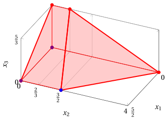
An optimal solution \({ \tilde{\boldsymbol x}}(\, LP \,)\) is:

\[ \tilde{x}_1=\dfrac{5}{2},~~ \tilde{x}_2=\dfrac{3}{2},~~ \tilde{x}_3=0 \]

the optimal value \(z(\, LP \,)\) is \(\dfrac{21}{2}.\)

In violet the first and the second vertex explored by the previous execution of the revised simplex algorithm (before reaching the optimal one depicted in blue).

Exercise 11.16: Revised simplex algorithm (P43)

Consider the following LP problem in canonical maximization form with \(n=3\) variables and \(m=2\) constraints:

\[ \begin{array}{rrrrrrrr} {\max} & {x_1} & {+} & {2}\, {x_2} & {+} & {7}\, {x_3} \\[2ex] \text{subject to} & {x_1} & & & {+} & {2}\, {x_3} & {\le} & {2} \\[2ex] & & & {x_2} & {+} & {2}\, {x_3} & {\le} & {2} \\[2ex] & {x_1,} & & {x_2,} & & {x_3} & {\ge} & {0} \end{array} \]

By introducing the slack variables, we get the following LP problem in standard maximization form with \(n+m=5\) variables and \(m=2\) constraints:

\[ \begin{array}{rrrrrrrrrrrr} {\max} & {x_1} & {+} & {2}\, {x_2} & {+} & {7}\, {x_3} \\[2ex] \text{subject to} & {x_1} & & & {+} & {2}\, {x_3} & {+} & {x_4} & & & {=} & {2} \\[2ex] & & & {x_2} & {+} & {2}\, {x_3} & & & {+} & {x_5} & {=} & {2} \\[2ex] & {x_1,} & & {x_2,} & & {x_3,} & & {x_4,} & & {x_5} & {\ge} & {0} \end{array} \]

Questions

• Execute the revised simplex algorithm to find an optimal solution of this LP problem using Bland's rule to select the pivot column and the pivot row.

Solution

We have:

\[ {\boldsymbol A}= \begin{pmatrix} 1 & 0 & 2 & 1 & 0\\ 0 & 1 & 2 & 0 & 1 \end{pmatrix} \quad {\boldsymbol b}= \begin{pmatrix} 2\\ 2 \end{pmatrix} \quad {\boldsymbol c}= \begin{pmatrix} 1\\ 2\\ 7\\ 0\\ 0 \end{pmatrix} \quad {\boldsymbol x}= \begin{pmatrix} x_1 \\ x_2 \\ x_3 \\ x_4 \\ x_5 \end{pmatrix} \]

• Initialization

  Since it is an LP problem in standard form obtained from an LP problem in canonical form with \(~{\boldsymbol b} \ge 0\) by adding the slack variables, the partition \(\pazocal{B}=\{4,5\}\) and \(\pazocal{N}=\{1,2,3\}\) is associated with the following basic feasible solution:

  \[ \begin{pmatrix} x_4 \\ x_5 \end{pmatrix} = \begin{pmatrix} 2\\ 2 \end{pmatrix} \text{ and } \begin{pmatrix} x_1 \\ x_2 \\ x_3 \end{pmatrix} = \begin{pmatrix} 0\\ 0\\ 0 \end{pmatrix} \]

• Iteration 1

  With \(\pazocal{B}= \{4,~~5\}\) and \(\pazocal{N}= \{1,~~2,~~3\}\), we have:

  \[ {\boldsymbol x}_{\pazocal{B}}= \begin{pmatrix} x_4 \\ x_5 \end{pmatrix} ~~ {\boldsymbol A}_{\pazocal{B}}= \begin{pmatrix} 1 & 0\\ 0 & 1 \end{pmatrix} ~~ {\boldsymbol c}_{\pazocal{B}}= \begin{pmatrix} 0\\ 0 \end{pmatrix} ~~ {{ \bar{\boldsymbol b}}}= \begin{pmatrix} 2\\ 2 \end{pmatrix} \]
  \[ {\boldsymbol x}_{\pazocal{N}}= \begin{pmatrix} x_1 \\ x_2 \\ x_3 \end{pmatrix} ~~ {\boldsymbol A}_{\pazocal{N}}= \begin{pmatrix} 1 & 0 & 2\\ 0 & 1 & 2 \end{pmatrix} ~~ {\boldsymbol c}_{\pazocal{N}}= \begin{pmatrix} 1\\ 2\\ 7 \end{pmatrix} \]

  Optimality check

  We solve \({\boldsymbol \pi} \; {\boldsymbol A}_{\pazocal{B}} = {\boldsymbol c}'_{\pazocal{B}}\) to compute \({\boldsymbol \pi} = {{{\boldsymbol c}'_{\pazocal{B}} \; {\boldsymbol A}_{\pazocal{B}}^{-1}}}\), first system of linear equations:

  \[\begin{equation*} \begin{cases} \begin{array}{rrrrr} {\pi_4} & & & {=} & {0} \\[2ex] & & {\pi_5} & {=} & {0} \end{array} \end{cases} \qquad {\boldsymbol \pi}= \begin{pmatrix} 0 & 0\\ \end{pmatrix} \end{equation*}\]

  We compute the basic feasible solution value \({\bar{z}} = {\boldsymbol \pi} \; {\boldsymbol b} = \begin{pmatrix} 0 & 0\\ \end{pmatrix} \begin{pmatrix} 2\\ 2 \end{pmatrix} = 0\)

  We compute the reduced costs \({{ \bar{\boldsymbol c}}'} = {{\boldsymbol c}'_{\pazocal{N}} - {\boldsymbol \pi} \; {\boldsymbol A}_{\pazocal{N}}}\):

  \[ \begin{aligned} {{ \bar{\boldsymbol c}}'} &= \begin{pmatrix} 1 & 2 & 7\\ \end{pmatrix} - \begin{pmatrix} 0 & 0\\ \end{pmatrix} \begin{pmatrix} 1 & 0 & 2\\ 0 & 1 & 2 \end{pmatrix} \\[1ex] &= \underbrace{ \begin{pmatrix} 1 & 2 & 7\\ \end{pmatrix} }_{{c_{1}~~~c_{2}~~~c_{3}}} - \underbrace{ \begin{pmatrix} 0 & 0 & 0\\ \end{pmatrix} }_{{\boldsymbol \pi}\;{\boldsymbol A}_{1} ~~{\boldsymbol \pi}\;{\boldsymbol A}_{2} ~~{\boldsymbol \pi}\;{\boldsymbol A}_{3}} = \underbrace{ \begin{pmatrix} 1 & 2 & 7\\ \end{pmatrix} }_{{\bar{c}_{1}~~~\bar{c}_{2}~~~\bar{c}_{3}}} \end{aligned} \]

  Not all reduced costs are non-positive then we perform a pivoting operation.

  Pivoting operation

  Since \({c}_{1} > {\boldsymbol \pi} \;{\boldsymbol A}_{1}\), \(x_1\) is the pivot column and we have \({\boldsymbol A}_{1} = \begin{pmatrix} 1\\ 0 \end{pmatrix}\)

  We solve \({\boldsymbol A}_{\pazocal{B}} \; {\boldsymbol d} = {\boldsymbol A}_{1}\) to compute \({\boldsymbol d}={ {\boldsymbol A}_{\pazocal{B}}^{-1}} {\boldsymbol A}_{1}\), second system of linear equations:

  \[\begin{equation*} \begin{cases} \begin{array}{rrrrr} {d_4} & & & {=} & {1} \\[2ex] & & {d_5} & {=} & {0} \end{array} \end{cases} \qquad {\boldsymbol d}= \begin{pmatrix} 1\\ 0 \end{pmatrix} \end{equation*}\]

  We have to find the largest \(t\) such that \({{ \bar{\boldsymbol b}}} - t \; {{\boldsymbol d}} \ge 0\):

  \[ \begin{cases} \underbrace{2 -t \cdot 1\ge 0}_{x_4 \ge 0} \end{cases} \qquad \begin{cases} t\le 2 \end{cases} \text{ then } t_{m}=2 \]

  Accordingly the value of the pivot column becomes \(t_{m}\), i.e., \(x_1=2\). The value of \(x_4\) becomes zero and \(x_4\) is the pivot row. The other basic variables take values \({ \bar{\boldsymbol b}} - t_{m} \; {\boldsymbol d}\), then we have:

  \[ x_5 = 2 - 2 \cdot 0 = 2 \]

• Iteration 2

  With \(\pazocal{B}= \{1,~~5\}\) and \(\pazocal{N}= \{2,~~3,~~4\}\), we have:

  \[ {\boldsymbol x}_{\pazocal{B}}= \begin{pmatrix} x_1 \\ x_5 \end{pmatrix} ~~ {\boldsymbol A}_{\pazocal{B}}= \begin{pmatrix} 1 & 0\\ 0 & 1 \end{pmatrix} ~~ {\boldsymbol c}_{\pazocal{B}}= \begin{pmatrix} 1\\ 0 \end{pmatrix} ~~ {{ \bar{\boldsymbol b}}}= \begin{pmatrix} 2\\ 2 \end{pmatrix} \]
  \[ {\boldsymbol x}_{\pazocal{N}}= \begin{pmatrix} x_2 \\ x_3 \\ x_4 \end{pmatrix} ~~ {\boldsymbol A}_{\pazocal{N}}= \begin{pmatrix} 0 & 2 & 1\\ 1 & 2 & 0 \end{pmatrix} ~~ {\boldsymbol c}_{\pazocal{N}}= \begin{pmatrix} 2\\ 7\\ 0 \end{pmatrix} \]

  Optimality check

  We solve \({\boldsymbol \pi} \; {\boldsymbol A}_{\pazocal{B}} = {\boldsymbol c}'_{\pazocal{B}}\) to compute \({\boldsymbol \pi} = {{{\boldsymbol c}'_{\pazocal{B}} \; {\boldsymbol A}_{\pazocal{B}}^{-1}}}\), first system of linear equations:

  \[\begin{equation*} \begin{cases} \begin{array}{rrrrr} {\pi_1} & & & {=} & {1} \\[2ex] & & {\pi_5} & {=} & {0} \end{array} \end{cases} \qquad {\boldsymbol \pi}= \begin{pmatrix} 1 & 0\\ \end{pmatrix} \end{equation*}\]

  We compute the basic feasible solution value \({\bar{z}} = {\boldsymbol \pi} \; {\boldsymbol b} = \begin{pmatrix} 1 & 0\\ \end{pmatrix} \begin{pmatrix} 2\\ 2 \end{pmatrix} = 2\)

  We compute the reduced costs \({{ \bar{\boldsymbol c}}'} = {{\boldsymbol c}'_{\pazocal{N}} - {\boldsymbol \pi} \; {\boldsymbol A}_{\pazocal{N}}}\):

  \[ \begin{aligned} {{ \bar{\boldsymbol c}}'} &= \begin{pmatrix} 2 & 7 & 0\\ \end{pmatrix} - \begin{pmatrix} 1 & 0\\ \end{pmatrix} \begin{pmatrix} 0 & 2 & 1\\ 1 & 2 & 0 \end{pmatrix} \\[1ex] &= \underbrace{ \begin{pmatrix} 2 & 7 & 0\\ \end{pmatrix} }_{{c_{2}~~~c_{3}~~~c_{4}}} - \underbrace{ \begin{pmatrix} 0 & 2 & 1\\ \end{pmatrix} }_{{\boldsymbol \pi}\;{\boldsymbol A}_{2} ~~{\boldsymbol \pi}\;{\boldsymbol A}_{3} ~~{\boldsymbol \pi}\;{\boldsymbol A}_{4}} = \underbrace{ \begin{pmatrix} 2 & 5 & -1\\ \end{pmatrix} }_{{\bar{c}_{2}~~~\bar{c}_{3}~~~\bar{c}_{4}}} \end{aligned} \]

  Not all reduced costs are non-positive then we perform a pivoting operation.

  Pivoting operation

  Since \({c}_{2} > {\boldsymbol \pi} \;{\boldsymbol A}_{2}\), \(x_2\) is the pivot column and we have \({\boldsymbol A}_{2} = \begin{pmatrix} 0\\ 1 \end{pmatrix}\)

  We solve \({\boldsymbol A}_{\pazocal{B}} \; {\boldsymbol d} = {\boldsymbol A}_{2}\) to compute \({\boldsymbol d}={ {\boldsymbol A}_{\pazocal{B}}^{-1}} {\boldsymbol A}_{2}\), second system of linear equations:

  \[\begin{equation*} \begin{cases} \begin{array}{rrrrr} {d_1} & & & {=} & {0} \\[2ex] & & {d_5} & {=} & {1} \end{array} \end{cases} \qquad {\boldsymbol d}= \begin{pmatrix} 0\\ 1 \end{pmatrix} \end{equation*}\]

  We have to find the largest \(t\) such that \({{ \bar{\boldsymbol b}}} - t \; {{\boldsymbol d}} \ge 0\):

  \[ \begin{cases} \underbrace{2 -t \cdot 1\ge 0}_{x_5 \ge 0} \end{cases} \qquad \begin{cases} t\le 2 \end{cases} \text{ then } t_{m}=2 \]

  Accordingly the value of the pivot column becomes \(t_{m}\), i.e., \(x_2=2\). The value of \(x_5\) becomes zero and \(x_5\) is the pivot row. The other basic variables take values \({ \bar{\boldsymbol b}} - t_{m} \; {\boldsymbol d}\), then we have:

  \[ x_1 = 2 - 2 \cdot 0 = 2 \]

• Iteration 3

  With \(\pazocal{B}= \{1,~~2\}\) and \(\pazocal{N}= \{3,~~4,~~5\}\), we have:

  \[ {\boldsymbol x}_{\pazocal{B}}= \begin{pmatrix} x_1 \\ x_2 \end{pmatrix} ~~ {\boldsymbol A}_{\pazocal{B}}= \begin{pmatrix} 1 & 0\\ 0 & 1 \end{pmatrix} ~~ {\boldsymbol c}_{\pazocal{B}}= \begin{pmatrix} 1\\ 2 \end{pmatrix} ~~ {{ \bar{\boldsymbol b}}}= \begin{pmatrix} 2\\ 2 \end{pmatrix} \]
  \[ {\boldsymbol x}_{\pazocal{N}}= \begin{pmatrix} x_3 \\ x_4 \\ x_5 \end{pmatrix} ~~ {\boldsymbol A}_{\pazocal{N}}= \begin{pmatrix} 2 & 1 & 0\\ 2 & 0 & 1 \end{pmatrix} ~~ {\boldsymbol c}_{\pazocal{N}}= \begin{pmatrix} 7\\ 0\\ 0 \end{pmatrix} \]

  Optimality check

  We solve \({\boldsymbol \pi} \; {\boldsymbol A}_{\pazocal{B}} = {\boldsymbol c}'_{\pazocal{B}}\) to compute \({\boldsymbol \pi} = {{{\boldsymbol c}'_{\pazocal{B}} \; {\boldsymbol A}_{\pazocal{B}}^{-1}}}\), first system of linear equations:

  \[\begin{equation*} \begin{cases} \begin{array}{rrrrr} {\pi_1} & & & {=} & {1} \\[2ex] & & {\pi_2} & {=} & {2} \end{array} \end{cases} \qquad {\boldsymbol \pi}= \begin{pmatrix} 1 & 2\\ \end{pmatrix} \end{equation*}\]

  We compute the basic feasible solution value \({\bar{z}} = {\boldsymbol \pi} \; {\boldsymbol b} = \begin{pmatrix} 1 & 2\\ \end{pmatrix} \begin{pmatrix} 2\\ 2 \end{pmatrix} = 6\)

  We compute the reduced costs \({{ \bar{\boldsymbol c}}'} = {{\boldsymbol c}'_{\pazocal{N}} - {\boldsymbol \pi} \; {\boldsymbol A}_{\pazocal{N}}}\):

  \[ \begin{aligned} {{ \bar{\boldsymbol c}}'} &= \begin{pmatrix} 7 & 0 & 0\\ \end{pmatrix} - \begin{pmatrix} 1 & 2\\ \end{pmatrix} \begin{pmatrix} 2 & 1 & 0\\ 2 & 0 & 1 \end{pmatrix} \\[1ex] &= \underbrace{ \begin{pmatrix} 7 & 0 & 0\\ \end{pmatrix} }_{{c_{3}~~~c_{4}~~~c_{5}}} - \underbrace{ \begin{pmatrix} 6 & 1 & 2\\ \end{pmatrix} }_{{\boldsymbol \pi}\;{\boldsymbol A}_{3} ~~{\boldsymbol \pi}\;{\boldsymbol A}_{4} ~~{\boldsymbol \pi}\;{\boldsymbol A}_{5}} = \underbrace{ \begin{pmatrix} 1 & -1 & -2\\ \end{pmatrix} }_{{\bar{c}_{3}~~~\bar{c}_{4}~~~\bar{c}_{5}}} \end{aligned} \]

  Not all reduced costs are non-positive then we perform a pivoting operation.

  Pivoting operation

  Since \({c}_{3} > {\boldsymbol \pi} \;{\boldsymbol A}_{3}\), \(x_3\) is the pivot column and we have \({\boldsymbol A}_{3} = \begin{pmatrix} 2\\ 2 \end{pmatrix}\)

  We solve \({\boldsymbol A}_{\pazocal{B}} \; {\boldsymbol d} = {\boldsymbol A}_{3}\) to compute \({\boldsymbol d}={ {\boldsymbol A}_{\pazocal{B}}^{-1}} {\boldsymbol A}_{3}\), second system of linear equations:

  \[\begin{equation*} \begin{cases} \begin{array}{rrrrr} {d_1} & & & {=} & {2} \\[2ex] & & {d_2} & {=} & {2} \end{array} \end{cases} \qquad {\boldsymbol d}= \begin{pmatrix} 2\\ 2 \end{pmatrix} \end{equation*}\]

  We have to find the largest \(t\) such that \({{ \bar{\boldsymbol b}}} - t \; {{\boldsymbol d}} \ge 0\):

  \[ \begin{cases} \underbrace{2 -t \cdot 2\ge 0}_{x_1 \ge 0} \\[2ex] \underbrace{2 -t \cdot 2\ge 0}_{x_2 \ge 0} \end{cases} \qquad \begin{cases} t\le 1 \\[2ex] t\le 1 \end{cases} \text{ then } t_{m}=1 \]

  Accordingly the value of the pivot column becomes \(t_{m}\), i.e., \(x_3=1\). The value of \(x_1\) becomes zero and \(x_1\) is the pivot row. The other basic variables take values \({ \bar{\boldsymbol b}} - t_{m} \; {\boldsymbol d}\), then we have:

  \[ x_2 = 2 - 1 \cdot 2 = 0 \]

• Iteration 4

  With \(\pazocal{B}= \{2,~~3\}\) and \(\pazocal{N}= \{1,~~4,~~5\}\), we have:

  \[ {\boldsymbol x}_{\pazocal{B}}= \begin{pmatrix} x_2 \\ x_3 \end{pmatrix} ~~ {\boldsymbol A}_{\pazocal{B}}= \begin{pmatrix} 0 & 2\\ 1 & 2 \end{pmatrix} ~~ {\boldsymbol c}_{\pazocal{B}}= \begin{pmatrix} 2\\ 7 \end{pmatrix} ~~ {{ \bar{\boldsymbol b}}}= \begin{pmatrix} 0\\ 1 \end{pmatrix} \]
  \[ {\boldsymbol x}_{\pazocal{N}}= \begin{pmatrix} x_1 \\ x_4 \\ x_5 \end{pmatrix} ~~ {\boldsymbol A}_{\pazocal{N}}= \begin{pmatrix} 1 & 1 & 0\\ 0 & 0 & 1 \end{pmatrix} ~~ {\boldsymbol c}_{\pazocal{N}}= \begin{pmatrix} 1\\ 0\\ 0 \end{pmatrix} \]

  Optimality check

  We solve \({\boldsymbol \pi} \; {\boldsymbol A}_{\pazocal{B}} = {\boldsymbol c}'_{\pazocal{B}}\) to compute \({\boldsymbol \pi} = {{{\boldsymbol c}'_{\pazocal{B}} \; {\boldsymbol A}_{\pazocal{B}}^{-1}}}\), first system of linear equations:

  \[\begin{equation*} \begin{cases} \begin{array}{rrrrr} & & {\pi_3} & {=} & {2} \\[2ex] {2}\, {\pi_2} & {+} & {2}\, {\pi_3} & {=} & {7} \end{array} \end{cases} \qquad {\boldsymbol \pi}= \begin{pmatrix} \dfrac{3}{2} & 2\\ \end{pmatrix} \end{equation*}\]

  We compute the basic feasible solution value \({\bar{z}} = {\boldsymbol \pi} \; {\boldsymbol b} = \begin{pmatrix} \dfrac{3}{2} & 2\\ \end{pmatrix} \begin{pmatrix} 2\\ 2 \end{pmatrix} = 7\)

  We compute the reduced costs \({{ \bar{\boldsymbol c}}'} = {{\boldsymbol c}'_{\pazocal{N}} - {\boldsymbol \pi} \; {\boldsymbol A}_{\pazocal{N}}}\):

  \[ \begin{aligned} {{ \bar{\boldsymbol c}}'} &= \begin{pmatrix} 1 & 0 & 0\\ \end{pmatrix} - \begin{pmatrix} \dfrac{3}{2} & 2\\ \end{pmatrix} \begin{pmatrix} 1 & 1 & 0\\ 0 & 0 & 1 \end{pmatrix} \\[1ex] &= \underbrace{ \begin{pmatrix} 1 & 0 & 0\\ \end{pmatrix} }_{{c_{1}~~~c_{4}~~~c_{5}}} - \underbrace{ \begin{pmatrix} \dfrac{3}{2} & \dfrac{3}{2} & 2\\ \end{pmatrix} }_{{\boldsymbol \pi}\;{\boldsymbol A}_{1} ~~{\boldsymbol \pi}\;{\boldsymbol A}_{4} ~~{\boldsymbol \pi}\;{\boldsymbol A}_{5}} = \underbrace{ \begin{pmatrix} -\dfrac{1}{2} & -\dfrac{3}{2} & -2\\ \end{pmatrix} }_{{\bar{c}_{1}~~~\bar{c}_{4}~~~\bar{c}_{5}}} \end{aligned} \]

  All reduced costs are non-positive, then the basic feasible solution

  \[ {\boldsymbol x}_{\pazocal{B}}= \begin{pmatrix} x_2 \\ x_3 \end{pmatrix}=\begin{pmatrix} 0\\ 1 \end{pmatrix} \text{ and } {\boldsymbol x}_{\pazocal{N}}= \begin{pmatrix} x_1 \\ x_4 \\ x_5 \end{pmatrix}=\begin{pmatrix} 0\\ 0\\ 0 \end{pmatrix} \]

  is an optimal solution of the LP problem and \({\bar{z}} = 7\) is the optimal solution value.

Graphical solution:

The feasible region of the LP problem (in canonical form) is the polyhedron shaded in red:

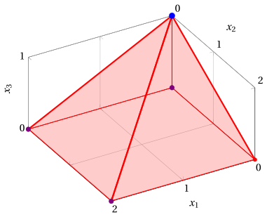
An optimal solution \({ \tilde{\boldsymbol x}}(\, LP \,)\) is:

\[ \tilde{x}_1=0,~~\tilde{x}_2=0,~~\tilde{x}_3=1 \]

the optimal value \(z(\, LP \,)\) is \(7.\)

In violet the first, the second and the third vertex explored by the previous execution of the revised simplex algorithm (before reaching the optimal one depicted in blue).

Exercise 11.17: Revised simplex algorithm (P44)

Consider the following LP problem in canonical maximization form with \(n=3\) variables and \(m=3\) constraints:

\[ \begin{array}{rrrrrrrr} {\max} & {x_1} & {+} & {2}\, {x_2} & {+} & {3}\, {x_3} \\[2ex] \text{subject to} & {x_1} & {+} & {2}\, {x_2} & {-} & {2}\, {x_3} & {\le} & {1} \\[2ex] & {2}\, {x_1} & {-} & {x_2} & {-} & {3}\, {x_3} & {\le} & {4} \\[2ex] & {x_1} & {+} & {2}\, {x_2} & {+} & {5}\, {x_3} & {\le} & {2} \\[2ex] & {x_1,} & & {x_2,} & & {x_3} & {\ge} & {0} \end{array} \]

By introducing the slack variables, we get the following LP problem in standard maximization form with \(n+m=6\) variables and \(m=3\) constraints:

\[ \begin{array}{rrcrcrcrcrcrcr} {\max} & {x_1} & {+} & {2}\, {x_2} & {+} & {3}\, {x_3} \\[2ex] \text{subject to} & {x_1} & {+} & {2}\, {x_2} & {-} & {2}\, {x_3} & {+} & {x_4} & & & & & {=} & {1} \\[2ex] & {2}\, {x_1} & {-} & {x_2} & {-} & {3}\, {x_3} & & & {+} & {x_5} & & & {=} & {4} \\[2ex] & {x_1} & {+} & {2}\, {x_2} & {+} & {5}\, {x_3} & & & & & {+} & {x_6} & {=} & {2} \\[2ex] & {x_1,} & & {x_2,} & & {x_3,} & & {x_4,} & & {x_5,} & & {x_6} & {\ge} & {0} \end{array} \]

Questions

• Execute the revised simplex algorithm to find an optimal solution of this LP problem using Bland's rule to select the pivot column and the pivot row.

Solution

We have:

\[ {\boldsymbol A}= \begin{pmatrix} 1 & 2 & -2 & 1 & 0 & 0\\ 2 & -1 & -3 & 0 & 1 & 0\\ 1 & 2 & 5 & 0 & 0 & 1 \end{pmatrix} \quad {\boldsymbol b}= \begin{pmatrix} 1\\ 4\\ 2 \end{pmatrix} \quad {\boldsymbol c}= \begin{pmatrix} 1\\ 2\\ 3\\ 0\\ 0\\ 0 \end{pmatrix} \quad {\boldsymbol x}= \begin{pmatrix} x_1 \\ x_2 \\ x_3 \\ x_4 \\ x_5 \\ x_6 \end{pmatrix} \]

• Initialization

  Since it is an LP problem in standard form obtained from an LP problem in canonical form with \(~{\boldsymbol b} \ge 0\) by adding the slack variables, the partition \(\pazocal{B}=\{4,5,6\}\) and \(\pazocal{N}=\{1,2,3\}\) is associated with the following basic feasible solution:

  \[ \begin{pmatrix} x_4 \\ x_5 \\ x_6 \end{pmatrix} = \begin{pmatrix} 1\\ 4\\ 2 \end{pmatrix} \text{ and } \begin{pmatrix} x_1 \\ x_2 \\ x_3 \end{pmatrix} = \begin{pmatrix} 0\\ 0\\ 0 \end{pmatrix} \]

• Iteration 1

  With \(\pazocal{B}= \{4,~~5,~~6\}\) and \(\pazocal{N}= \{1,~~2,~~3\}\), we have:

  \[ {\boldsymbol x}_{\pazocal{B}}= \begin{pmatrix} x_4 \\ x_5 \\ x_6 \end{pmatrix} ~~ {\boldsymbol A}_{\pazocal{B}}= \begin{pmatrix} 1 & 0 & 0\\ 0 & 1 & 0\\ 0 & 0 & 1 \end{pmatrix} ~~ {\boldsymbol c}_{\pazocal{B}}= \begin{pmatrix} 0\\ 0\\ 0 \end{pmatrix} ~~ {{ \bar{\boldsymbol b}}}= \begin{pmatrix} 1\\ 4\\ 2 \end{pmatrix} \]
  \[ {\boldsymbol x}_{\pazocal{N}}= \begin{pmatrix} x_1 \\ x_2 \\ x_3 \end{pmatrix} ~~ {\boldsymbol A}_{\pazocal{N}}= \begin{pmatrix} 1 & 2 & -2\\ 2 & -1 & -3\\ 1 & 2 & 5 \end{pmatrix} ~~ {\boldsymbol c}_{\pazocal{N}}= \begin{pmatrix} 1\\ 2\\ 3 \end{pmatrix} \]

  Optimality check

  We solve \({\boldsymbol \pi} \; {\boldsymbol A}_{\pazocal{B}} = {\boldsymbol c}'_{\pazocal{B}}\) to compute \({\boldsymbol \pi} = {{{\boldsymbol c}'_{\pazocal{B}} \; {\boldsymbol A}_{\pazocal{B}}^{-1}}}\), first system of linear equations:

  \[\begin{equation*} \begin{cases} \begin{array}{rrrrrrr} {\pi_4} & & & & & {=} & {0} \\[2ex] & & {\pi_5} & & & {=} & {0} \\[2ex] & & & & {\pi_6} & {=} & {0} \end{array} \end{cases} \qquad {\boldsymbol \pi}= \begin{pmatrix} 0 & 0 & 0\\ \end{pmatrix} \end{equation*}\]

  We compute the basic feasible solution value \({\bar{z}} = {\boldsymbol \pi} \; {\boldsymbol b} = \begin{pmatrix} 0 & 0 & 0\\ \end{pmatrix} \begin{pmatrix} 1\\ 4\\ 2 \end{pmatrix} = 0\)

  We compute the reduced costs \({{ \bar{\boldsymbol c}}'} = {{\boldsymbol c}'_{\pazocal{N}} - {\boldsymbol \pi} \; {\boldsymbol A}_{\pazocal{N}}}\):

  \[ \begin{aligned} {{ \bar{\boldsymbol c}}'} &= \begin{pmatrix} 1 & 2 & 3\\ \end{pmatrix} - \begin{pmatrix} 0 & 0 & 0\\ \end{pmatrix} \begin{pmatrix} 1 & 2 & -2\\ 2 & -1 & -3\\ 1 & 2 & 5 \end{pmatrix} \\[1ex] &= \underbrace{ \begin{pmatrix} 1 & 2 & 3\\ \end{pmatrix} }_{{c_{1}~~~c_{2}~~~c_{3}}} - \underbrace{ \begin{pmatrix} 0 & 0 & 0\\ \end{pmatrix} }_{{\boldsymbol \pi}\;{\boldsymbol A}_{1} ~~{\boldsymbol \pi}\;{\boldsymbol A}_{2} ~~{\boldsymbol \pi}\;{\boldsymbol A}_{3}} = \underbrace{ \begin{pmatrix} 1 & 2 & 3\\ \end{pmatrix} }_{{\bar{c}_{1}~~~\bar{c}_{2}~~~\bar{c}_{3}}} \end{aligned} \]

  Not all reduced costs are non-positive then we perform a pivoting operation.

  Pivoting operation

  Since \({c}_{1} > {\boldsymbol \pi} \;{\boldsymbol A}_{1}\), \(x_1\) is the pivot column and we have \({\boldsymbol A}_{1} = \begin{pmatrix} 1\\ 2\\ 1 \end{pmatrix}\)

  We solve \({\boldsymbol A}_{\pazocal{B}} \; {\boldsymbol d} = {\boldsymbol A}_{1}\) to compute \({\boldsymbol d}={ {\boldsymbol A}_{\pazocal{B}}^{-1}} {\boldsymbol A}_{1}\), second system of linear equations:

  \[\begin{equation*} \begin{cases} \begin{array}{rrrrrrr} {d_4} & & & & & {=} & {1} \\[2ex] & & {d_5} & & & {=} & {2} \\[2ex] & & & & {d_6} & {=} & {1} \end{array} \end{cases} \qquad {\boldsymbol d}= \begin{pmatrix} 1\\ 2\\ 1 \end{pmatrix} \end{equation*}\]

  We have to find the largest \(t\) such that \({{ \bar{\boldsymbol b}}} - t \; {{\boldsymbol d}} \ge 0\):

  \[ \begin{cases} \underbrace{1 -t \cdot 1\ge 0}_{x_4 \ge 0} \\[2ex] \underbrace{4 -t \cdot 2\ge 0}_{x_5 \ge 0} \\[2ex] \underbrace{2 -t \cdot 1\ge 0}_{x_6 \ge 0} \end{cases} \qquad \begin{cases} t\le 1 \\[2ex] t\le 2 \\[2ex] t\le 2 \end{cases} \text{ then } t_{m}=1 \]

  Accordingly the value of the pivot column becomes \(t_{m}\), i.e., \(x_1=1\). The value of \(x_4\) becomes zero and \(x_4\) is the pivot row. The other basic variables take values \({ \bar{\boldsymbol b}} - t_{m} \; {\boldsymbol d}\), then we have:

  \[ \begin{aligned} x_5 &= 4 - 1 \cdot 2 = 2 \\[2ex] x_6 &= 2 - 1 \cdot 1 = 1 \end{aligned} \]

• Iteration 2

  With \(\pazocal{B}= \{1,~~5,~~6\}\) and \(\pazocal{N}= \{2,~~3,~~4\}\), we have:

  \[ {\boldsymbol x}_{\pazocal{B}}= \begin{pmatrix} x_1 \\ x_5 \\ x_6 \end{pmatrix} ~~ {\boldsymbol A}_{\pazocal{B}}= \begin{pmatrix} 1 & 0 & 0\\ 2 & 1 & 0\\ 1 & 0 & 1 \end{pmatrix} ~~ {\boldsymbol c}_{\pazocal{B}}= \begin{pmatrix} 1\\ 0\\ 0 \end{pmatrix} ~~ {{ \bar{\boldsymbol b}}}= \begin{pmatrix} 1\\ 2\\ 1 \end{pmatrix} \]
  \[ {\boldsymbol x}_{\pazocal{N}}= \begin{pmatrix} x_2 \\ x_3 \\ x_4 \end{pmatrix} ~~ {\boldsymbol A}_{\pazocal{N}}= \begin{pmatrix} 2 & -2 & 1\\ -1 & -3 & 0\\ 2 & 5 & 0 \end{pmatrix} ~~ {\boldsymbol c}_{\pazocal{N}}= \begin{pmatrix} 2\\ 3\\ 0 \end{pmatrix} \]

  Optimality check

  We solve \({\boldsymbol \pi} \; {\boldsymbol A}_{\pazocal{B}} = {\boldsymbol c}'_{\pazocal{B}}\) to compute \({\boldsymbol \pi} = {{{\boldsymbol c}'_{\pazocal{B}} \; {\boldsymbol A}_{\pazocal{B}}^{-1}}}\), first system of linear equations:

  \[\begin{equation*} \begin{cases} \begin{array}{rrrrrrr} {\pi_1} & {+} & {2}\, {\pi_5} & {+} & {\pi_6} & {=} & {1} \\[2ex] & & {\pi_5} & & & {=} & {0} \\[2ex] & & & & {\pi_6} & {=} & {0} \end{array} \end{cases} \qquad {\boldsymbol \pi}= \begin{pmatrix} 1 & 0 & 0\\ \end{pmatrix} \end{equation*}\]

  We compute the basic feasible solution value \({\bar{z}} = {\boldsymbol \pi} \; {\boldsymbol b} = \begin{pmatrix} 1 & 0 & 0\\ \end{pmatrix} \begin{pmatrix} 1\\ 4\\ 2 \end{pmatrix} = 1\)

  We compute the reduced costs \({{ \bar{\boldsymbol c}}'} = {{\boldsymbol c}'_{\pazocal{N}} - {\boldsymbol \pi} \; {\boldsymbol A}_{\pazocal{N}}}\):

  \[ \begin{aligned} {{ \bar{\boldsymbol c}}'} &= \begin{pmatrix} 2 & 3 & 0\\ \end{pmatrix} - \begin{pmatrix} 1 & 0 & 0\\ \end{pmatrix} \begin{pmatrix} 2 & -2 & 1\\ -1 & -3 & 0\\ 2 & 5 & 0 \end{pmatrix} \\[1ex] &= \underbrace{ \begin{pmatrix} 2 & 3 & 0\\ \end{pmatrix} }_{{c_{2}~~~c_{3}~~~c_{4}}} - \underbrace{ \begin{pmatrix} 2 & -2 & 1\\ \end{pmatrix} }_{{\boldsymbol \pi}\;{\boldsymbol A}_{2} ~~{\boldsymbol \pi}\;{\boldsymbol A}_{3} ~~{\boldsymbol \pi}\;{\boldsymbol A}_{4}} = \underbrace{ \begin{pmatrix} 0 & 5 & -1\\ \end{pmatrix} }_{{\bar{c}_{2}~~~\bar{c}_{3}~~~\bar{c}_{4}}} \end{aligned} \]

  Not all reduced costs are non-positive then we perform a pivoting operation.

  Pivoting operation

  Since \({c}_{3} > {\boldsymbol \pi} \;{\boldsymbol A}_{3}\), \(x_3\) is the pivot column and we have \({\boldsymbol A}_{3} = \begin{pmatrix} -2\\ -3\\ 5 \end{pmatrix}\)

  We solve \({\boldsymbol A}_{\pazocal{B}} \; {\boldsymbol d} = {\boldsymbol A}_{3}\) to compute \({\boldsymbol d}={ {\boldsymbol A}_{\pazocal{B}}^{-1}} {\boldsymbol A}_{3}\), second system of linear equations:

  \[\begin{equation*} \begin{cases} \begin{array}{rrrrrrr} {d_1} & & & & & {=} & {-2} \\[2ex] {2}\, {d_1} & {+} & {d_5} & & & {=} & {-3} \\[2ex] {d_1} & & & {+} & {d_6} & {=} & {5} \end{array} \end{cases} \qquad {\boldsymbol d}= \begin{pmatrix} -2\\ 1\\ 7 \end{pmatrix} \end{equation*}\]

  We have to find the largest \(t\) such that \({{ \bar{\boldsymbol b}}} - t \; {{\boldsymbol d}} \ge 0\):

  \[ \begin{cases} \underbrace{1 -t \cdot \left( -2\right)\ge 0}_{x_1 \ge 0} \\[2ex] \underbrace{2 -t \cdot 1\ge 0}_{x_5 \ge 0} \\[2ex] \underbrace{1 -t \cdot 7\ge 0}_{x_6 \ge 0} \end{cases} \qquad \begin{cases} t\ge -\dfrac{1}{2} \\[2ex] t\le 2 \\[2ex] t\le \dfrac{1}{7} \end{cases} \text{ then } t_{m}=\dfrac{1}{7} \]

  Accordingly the value of the pivot column becomes \(t_{m}\), i.e., \(x_3=\dfrac{1}{7}\). The value of \(x_6\) becomes zero and \(x_6\) is the pivot row. The other basic variables take values \({ \bar{\boldsymbol b}} - t_{m} \; {\boldsymbol d}\), then we have:

  \[ \begin{aligned} x_1 &= 1 - \dfrac{1}{7} \cdot \left( -2\right) = \dfrac{9}{7} \\[2ex] x_5 &= 2 - \dfrac{1}{7} \cdot 1 = \dfrac{13}{7} \end{aligned} \]

• Iteration 3

  With \(\pazocal{B}= \{1,~~3,~~5\}\) and \(\pazocal{N}= \{2,~~4,~~6\}\), we have:

  \[ {\boldsymbol x}_{\pazocal{B}}= \begin{pmatrix} x_1 \\ x_3 \\ x_5 \end{pmatrix} ~~ {\boldsymbol A}_{\pazocal{B}}= \begin{pmatrix} 1 & -2 & 0\\ 2 & -3 & 1\\ 1 & 5 & 0 \end{pmatrix} ~~ {\boldsymbol c}_{\pazocal{B}}= \begin{pmatrix} 1\\ 3\\ 0 \end{pmatrix} ~~ {{ \bar{\boldsymbol b}}}= \begin{pmatrix} \dfrac{9}{7}\\[2ex] \dfrac{1}{7}\\[2ex] \dfrac{13}{7} \end{pmatrix} \]
  \[ {\boldsymbol x}_{\pazocal{N}}= \begin{pmatrix} x_2 \\ x_4 \\ x_6 \end{pmatrix} ~~ {\boldsymbol A}_{\pazocal{N}}= \begin{pmatrix} 2 & 1 & 0\\ -1 & 0 & 0\\ 2 & 0 & 1 \end{pmatrix} ~~ {\boldsymbol c}_{\pazocal{N}}= \begin{pmatrix} 2\\ 0\\ 0 \end{pmatrix} \]

  Optimality check

  We solve \({\boldsymbol \pi} \; {\boldsymbol A}_{\pazocal{B}} = {\boldsymbol c}'_{\pazocal{B}}\) to compute \({\boldsymbol \pi} = {{{\boldsymbol c}'_{\pazocal{B}} \; {\boldsymbol A}_{\pazocal{B}}^{-1}}}\), first system of linear equations:

  \[\begin{equation*} \begin{cases} \begin{array}{rrrrrrr} {\pi_1} & {+} & {2}\, {\pi_3} & {+} & {\pi_5} & {=} & {1} \\[2ex] {-2}\, {\pi_1} & {-} & {3}\, {\pi_3} & {+} & {5}\, {\pi_5} & {=} & {3} \\[2ex] & & {\pi_3} & & & {=} & {0} \end{array} \end{cases} \qquad {\boldsymbol \pi}= \begin{pmatrix} \dfrac{2}{7} & 0 & \dfrac{5}{7}\\ \end{pmatrix} \end{equation*}\]

  We compute the basic feasible solution value \({\bar{z}} = {\boldsymbol \pi} \; {\boldsymbol b} = \begin{pmatrix} \dfrac{2}{7} & 0 & \dfrac{5}{7}\\ \end{pmatrix} \begin{pmatrix} 1\\ 4\\ 2 \end{pmatrix} = \dfrac{12}{7}\)

  We compute the reduced costs \({{ \bar{\boldsymbol c}}'} = {{\boldsymbol c}'_{\pazocal{N}} - {\boldsymbol \pi} \; {\boldsymbol A}_{\pazocal{N}}}\):

  \[ \begin{aligned} {{ \bar{\boldsymbol c}}'} &= \begin{pmatrix} 2 & 0 & 0\\ \end{pmatrix} - \begin{pmatrix} \dfrac{2}{7} & 0 & \dfrac{5}{7}\\ \end{pmatrix} \begin{pmatrix} 2 & 1 & 0\\ -1 & 0 & 0\\ 2 & 0 & 1 \end{pmatrix} \\[1ex] &= \underbrace{ \begin{pmatrix} 2 & 0 & 0\\ \end{pmatrix} }_{{c_{2}~~~c_{4}~~~c_{6}}} - \underbrace{ \begin{pmatrix} 2 & \dfrac{2}{7} & \dfrac{5}{7}\\ \end{pmatrix} }_{{\boldsymbol \pi}\;{\boldsymbol A}_{2} ~~{\boldsymbol \pi}\;{\boldsymbol A}_{4} ~~{\boldsymbol \pi}\;{\boldsymbol A}_{6}} = \underbrace{ \begin{pmatrix} 0 & -\dfrac{2}{7} & -\dfrac{5}{7}\\ \end{pmatrix} }_{{\bar{c}_{2}~~~\bar{c}_{4}~~~\bar{c}_{6}}} \end{aligned} \]

  All reduced costs are non-positive, then the basic feasible solution

  \[ {\boldsymbol x}_{\pazocal{B}}= \begin{pmatrix} x_1 \\ x_3 \\ x_5 \end{pmatrix}=\begin{pmatrix} \dfrac{9}{7}\\[2ex] \dfrac{1}{7}\\[2ex] \dfrac{13}{7} \end{pmatrix} \text{ and } {\boldsymbol x}_{\pazocal{N}}= \begin{pmatrix} x_2 \\ x_4 \\ x_6 \end{pmatrix}=\begin{pmatrix} 0\\ 0\\ 0 \end{pmatrix} \]

  is an optimal solution of the LP problem and \({\bar{z}} = \dfrac{12}{7}\) is the optimal solution value.

• Multiple optimal solutions

  The optimal solution is not unique: in the final basis the non-basic variable \(x_2\) has reduced cost \(\bar c_{2} = 0\), and every point of the edge joining \(\left(\dfrac{9}{7},~0,~\dfrac{1}{7}\right)\) and \(\left(0,~\dfrac{9}{14},~\dfrac{1}{7}\right)\) is optimal, with value \(\dfrac{12}{7}\).

Graphical solution:

The feasible region of the LP problem (in canonical form) is the polyhedron shaded in red:

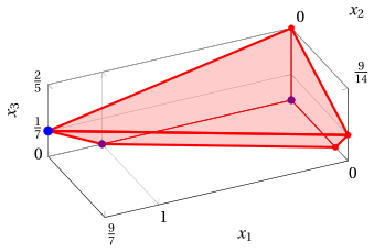
An optimal solution \({ \tilde{\boldsymbol x}}(\, LP \,)\) is:

\[ \tilde{x}_1=\dfrac{9}{7},~~\tilde{x}_2=0,~~\tilde{x}_3=\dfrac{1}{7} \]

the optimal value \(z(\, LP \,)\) is \(\dfrac{12}{7}.\)

In violet the first and the second vertex explored by the previous execution of the revised simplex algorithm (before reaching the optimal one depicted in blue).

Exercise 11.18: Revised simplex algorithm (P45)

Consider the following LP problem in canonical maximization form with \(n=3\) variables and \(m=2\) constraints:

\[ \begin{array}{rrrrrrrr} {\max} & {4}\, {x_1} & {-} & {13}\, {x_2} & {+} & {7}\, {x_3} \\[2ex] \text{subject to} & {3}\, {x_1} & {+} & {2}\, {x_2} & {+} & {5}\, {x_3} & {\le} & {5} \\[2ex] & {x_1} & {-} & {3}\, {x_2} & {+} & {5}\, {x_3} & {\le} & {3} \\[2ex] & {x_1,} & & {x_2,} & & {x_3} & {\ge} & {0} \end{array} \]

By introducing the slack variables, we get the following LP problem in standard maximization form with \(n+m=5\) variables and \(m=2\) constraints:

\[ \begin{array}{rrrrrrrrrrrr} {\max} & {4}\, {x_1} & {-} & {13}\, {x_2} & {+} & {7}\, {x_3} \\[2ex] \text{subject to} & {3}\, {x_1} & {+} & {2}\, {x_2} & {+} & {5}\, {x_3} & {+} & {x_4} & & & {=} & {5} \\[2ex] & {x_1} & {-} & {3}\, {x_2} & {+} & {5}\, {x_3} & & & {+} & {x_5} & {=} & {3} \\[2ex] & {x_1,} & & {x_2,} & & {x_3,} & & {x_4,} & & {x_5} & {\ge} & {0} \end{array} \]

Questions

• Execute the revised simplex algorithm to find an optimal solution of this LP problem using Bland's rule to select the pivot column and the pivot row.

Solution

We have:

\[ {\boldsymbol A}= \begin{pmatrix} 3 & 2 & 5 & 1 & 0\\ 1 & -3 & 5 & 0 & 1 \end{pmatrix} \quad {\boldsymbol b}= \begin{pmatrix} 5\\ 3 \end{pmatrix} \quad {\boldsymbol c}= \begin{pmatrix} 4\\ -13\\ 7\\ 0\\ 0 \end{pmatrix} \quad {\boldsymbol x}= \begin{pmatrix} x_1 \\ x_2 \\ x_3 \\ x_4 \\ x_5 \end{pmatrix} \]

• Initialization

  Since it is an LP problem in standard form obtained from an LP problem in canonical form with \(~{\boldsymbol b} \ge 0\) by adding the slack variables, the partition \(\pazocal{B}=\{4,5\}\) and \(\pazocal{N}=\{1,2,3\}\) is associated with the following basic feasible solution:

  \[ \begin{pmatrix} x_4 \\ x_5 \end{pmatrix} = \begin{pmatrix} 5\\ 3 \end{pmatrix} \text{ and } \begin{pmatrix} x_1 \\ x_2 \\ x_3 \end{pmatrix} = \begin{pmatrix} 0\\ 0\\ 0 \end{pmatrix} \]

• Iteration 1

  With \(\pazocal{B}= \{4,~~5\}\) and \(\pazocal{N}= \{1,~~2,~~3\}\), we have:

  \[ {\boldsymbol x}_{\pazocal{B}}= \begin{pmatrix} x_4 \\ x_5 \end{pmatrix} ~~ {\boldsymbol A}_{\pazocal{B}}= \begin{pmatrix} 1 & 0\\ 0 & 1 \end{pmatrix} ~~ {\boldsymbol c}_{\pazocal{B}}= \begin{pmatrix} 0\\ 0 \end{pmatrix} ~~ {{ \bar{\boldsymbol b}}}= \begin{pmatrix} 5\\ 3 \end{pmatrix} \]
  \[ {\boldsymbol x}_{\pazocal{N}}= \begin{pmatrix} x_1 \\ x_2 \\ x_3 \end{pmatrix} ~~ {\boldsymbol A}_{\pazocal{N}}= \begin{pmatrix} 3 & 2 & 5\\ 1 & -3 & 5 \end{pmatrix} ~~ {\boldsymbol c}_{\pazocal{N}}= \begin{pmatrix} 4\\ -13\\ 7 \end{pmatrix} \]

  Optimality check

  We solve \({\boldsymbol \pi} \; {\boldsymbol A}_{\pazocal{B}} = {\boldsymbol c}'_{\pazocal{B}}\) to compute \({\boldsymbol \pi} = {{{\boldsymbol c}'_{\pazocal{B}} \; {\boldsymbol A}_{\pazocal{B}}^{-1}}}\), first system of linear equations:

  \[\begin{equation*} \begin{cases} \begin{array}{rrrrr} {\pi_4} & & & {=} & {0} \\[2ex] & & {\pi_5} & {=} & {0} \end{array} \end{cases} \qquad {\boldsymbol \pi}= \begin{pmatrix} 0 & 0\\ \end{pmatrix} \end{equation*}\]

  We compute the basic feasible solution value \({\bar{z}} = {\boldsymbol \pi} \; {\boldsymbol b} = \begin{pmatrix} 0 & 0\\ \end{pmatrix} \begin{pmatrix} 5\\ 3 \end{pmatrix} = 0\)

  We compute the reduced costs \({{ \bar{\boldsymbol c}}'} = {{\boldsymbol c}'_{\pazocal{N}} - {\boldsymbol \pi} \; {\boldsymbol A}_{\pazocal{N}}}\):

  \[ \begin{aligned} {{ \bar{\boldsymbol c}}'} &= \begin{pmatrix} 4 & -13 & 7\\ \end{pmatrix} - \begin{pmatrix} 0 & 0\\ \end{pmatrix} \begin{pmatrix} 3 & 2 & 5\\ 1 & -3 & 5 \end{pmatrix} \\[1ex] &= \underbrace{ \begin{pmatrix} 4 & -13 & 7\\ \end{pmatrix} }_{{c_{1}~~~c_{2}~~~c_{3}}} - \underbrace{ \begin{pmatrix} 0 & 0 & 0\\ \end{pmatrix} }_{{\boldsymbol \pi}\;{\boldsymbol A}_{1} ~~{\boldsymbol \pi}\;{\boldsymbol A}_{2} ~~{\boldsymbol \pi}\;{\boldsymbol A}_{3}} = \underbrace{ \begin{pmatrix} 4 & -13 & 7\\ \end{pmatrix} }_{{\bar{c}_{1}~~~\bar{c}_{2}~~~\bar{c}_{3}}} \end{aligned} \]

  Not all reduced costs are non-positive then we perform a pivoting operation.

  Pivoting operation

  Since \({c}_{1} > {\boldsymbol \pi} \;{\boldsymbol A}_{1}\), \(x_1\) is the pivot column and we have \({\boldsymbol A}_{1} = \begin{pmatrix} 3\\ 1 \end{pmatrix}\)

  We solve \({\boldsymbol A}_{\pazocal{B}} \; {\boldsymbol d} = {\boldsymbol A}_{1}\) to compute \({\boldsymbol d}={ {\boldsymbol A}_{\pazocal{B}}^{-1}} {\boldsymbol A}_{1}\), second system of linear equations:

  \[\begin{equation*} \begin{cases} \begin{array}{rrrrr} {d_4} & & & {=} & {3} \\[2ex] & & {d_5} & {=} & {1} \end{array} \end{cases} \qquad {\boldsymbol d}= \begin{pmatrix} 3\\ 1 \end{pmatrix} \end{equation*}\]

  We have to find the largest \(t\) such that \({{ \bar{\boldsymbol b}}} - t \; {{\boldsymbol d}} \ge 0\):

  \[ \begin{cases} \underbrace{5 -t \cdot 3\ge 0}_{x_4 \ge 0} \\[2ex] \underbrace{3 -t \cdot 1\ge 0}_{x_5 \ge 0} \end{cases} \qquad \begin{cases} t\le \dfrac{5}{3} \\[2ex] t\le 3 \end{cases} \text{ then } t_{m}=\dfrac{5}{3} \]

  Accordingly the value of the pivot column becomes \(t_{m}\), i.e., \(x_1=\dfrac{5}{3}\). The value of \(x_4\) becomes zero and \(x_4\) is the pivot row. The other basic variables take values \({ \bar{\boldsymbol b}} - t_{m} \; {\boldsymbol d}\), then we have:

  \[ x_5 = 3 - \dfrac{5}{3} \cdot 1 = \dfrac{4}{3} \]

• Iteration 2

  With \(\pazocal{B}= \{1,~~5\}\) and \(\pazocal{N}= \{2,~~3,~~4\}\), we have:

  \[ {\boldsymbol x}_{\pazocal{B}}= \begin{pmatrix} x_1 \\ x_5 \end{pmatrix} ~~ {\boldsymbol A}_{\pazocal{B}}= \begin{pmatrix} 3 & 0\\ 1 & 1 \end{pmatrix} ~~ {\boldsymbol c}_{\pazocal{B}}= \begin{pmatrix} 4\\ 0 \end{pmatrix} ~~ {{ \bar{\boldsymbol b}}}= \begin{pmatrix} \dfrac{5}{3}\\[2ex] \dfrac{4}{3} \end{pmatrix} \]
  \[ {\boldsymbol x}_{\pazocal{N}}= \begin{pmatrix} x_2 \\ x_3 \\ x_4 \end{pmatrix} ~~ {\boldsymbol A}_{\pazocal{N}}= \begin{pmatrix} 2 & 5 & 1\\ -3 & 5 & 0 \end{pmatrix} ~~ {\boldsymbol c}_{\pazocal{N}}= \begin{pmatrix} -13\\ 7\\ 0 \end{pmatrix} \]

  Optimality check

  We solve \({\boldsymbol \pi} \; {\boldsymbol A}_{\pazocal{B}} = {\boldsymbol c}'_{\pazocal{B}}\) to compute \({\boldsymbol \pi} = {{{\boldsymbol c}'_{\pazocal{B}} \; {\boldsymbol A}_{\pazocal{B}}^{-1}}}\), first system of linear equations:

  \[\begin{equation*} \begin{cases} \begin{array}{rrrrr} {3}\, {\pi_1} & {+} & {\pi_5} & {=} & {4} \\[2ex] & & {\pi_5} & {=} & {0} \end{array} \end{cases} \qquad {\boldsymbol \pi}= \begin{pmatrix} \dfrac{4}{3} & 0\\ \end{pmatrix} \end{equation*}\]

  We compute the basic feasible solution value \({\bar{z}} = {\boldsymbol \pi} \; {\boldsymbol b} = \begin{pmatrix} \dfrac{4}{3} & 0\\ \end{pmatrix} \begin{pmatrix} 5\\ 3 \end{pmatrix} = \dfrac{20}{3}\)

  We compute the reduced costs \({{ \bar{\boldsymbol c}}'} = {{\boldsymbol c}'_{\pazocal{N}} - {\boldsymbol \pi} \; {\boldsymbol A}_{\pazocal{N}}}\):

  \[ \begin{aligned} {{ \bar{\boldsymbol c}}'} &= \begin{pmatrix} -13 & 7 & 0\\ \end{pmatrix} - \begin{pmatrix} \dfrac{4}{3} & 0\\ \end{pmatrix} \begin{pmatrix} 2 & 5 & 1\\ -3 & 5 & 0 \end{pmatrix} \\[1ex] &= \underbrace{ \begin{pmatrix} -13 & 7 & 0\\ \end{pmatrix} }_{{c_{2}~~~c_{3}~~~c_{4}}} - \underbrace{ \begin{pmatrix} \dfrac{8}{3} & \dfrac{20}{3} & \dfrac{4}{3}\\ \end{pmatrix} }_{{\boldsymbol \pi}\;{\boldsymbol A}_{2} ~~{\boldsymbol \pi}\;{\boldsymbol A}_{3} ~~{\boldsymbol \pi}\;{\boldsymbol A}_{4}} = \underbrace{ \begin{pmatrix} -\dfrac{47}{3} & \dfrac{1}{3} & -\dfrac{4}{3}\\ \end{pmatrix} }_{{\bar{c}_{2}~~~\bar{c}_{3}~~~\bar{c}_{4}}} \end{aligned} \]

  Not all reduced costs are non-positive then we perform a pivoting operation.

  Pivoting operation

  Since \({c}_{3} > {\boldsymbol \pi} \;{\boldsymbol A}_{3}\), \(x_3\) is the pivot column and we have \({\boldsymbol A}_{3} = \begin{pmatrix} 5\\ 5 \end{pmatrix}\)

  We solve \({\boldsymbol A}_{\pazocal{B}} \; {\boldsymbol d} = {\boldsymbol A}_{3}\) to compute \({\boldsymbol d}={ {\boldsymbol A}_{\pazocal{B}}^{-1}} {\boldsymbol A}_{3}\), second system of linear equations:

  \[\begin{equation*} \begin{cases} \begin{array}{rrrrr} {3}\, {d_1} & & & {=} & {5} \\[2ex] {d_1} & {+} & {d_5} & {=} & {5} \end{array} \end{cases} \qquad {\boldsymbol d}= \begin{pmatrix} \dfrac{5}{3}\\[2ex] \dfrac{10}{3} \end{pmatrix} \end{equation*}\]

  We have to find the largest \(t\) such that \({{ \bar{\boldsymbol b}}} - t \; {{\boldsymbol d}} \ge 0\):

  \[ \begin{cases} \underbrace{\dfrac{5}{3} -t \cdot \dfrac{5}{3}\ge 0}_{x_1 \ge 0} \\[2ex] \underbrace{\dfrac{4}{3} -t \cdot \dfrac{10}{3}\ge 0}_{x_5 \ge 0} \end{cases} \qquad \begin{cases} t\le 1 \\[2ex] t\le \dfrac{2}{5} \end{cases} \text{ then } t_{m}=\dfrac{2}{5} \]

  Accordingly the value of the pivot column becomes \(t_{m}\), i.e., \(x_3=\dfrac{2}{5}\). The value of \(x_5\) becomes zero and \(x_5\) is the pivot row. The other basic variables take values \({ \bar{\boldsymbol b}} - t_{m} \; {\boldsymbol d}\), then we have:

  \[ x_1 = \dfrac{5}{3} - \dfrac{2}{5} \cdot \dfrac{5}{3} = 1 \]

• Iteration 3

  With \(\pazocal{B}= \{1,~~3\}\) and \(\pazocal{N}= \{2,~~4,~~5\}\), we have:

  \[ {\boldsymbol x}_{\pazocal{B}}= \begin{pmatrix} x_1 \\ x_3 \end{pmatrix} ~~ {\boldsymbol A}_{\pazocal{B}}= \begin{pmatrix} 3 & 5\\ 1 & 5 \end{pmatrix} ~~ {\boldsymbol c}_{\pazocal{B}}= \begin{pmatrix} 4\\ 7 \end{pmatrix} ~~ {{ \bar{\boldsymbol b}}}= \begin{pmatrix} 1\\[2ex] \dfrac{2}{5} \end{pmatrix} \]
  \[ {\boldsymbol x}_{\pazocal{N}}= \begin{pmatrix} x_2 \\ x_4 \\ x_5 \end{pmatrix} ~~ {\boldsymbol A}_{\pazocal{N}}= \begin{pmatrix} 2 & 1 & 0\\ -3 & 0 & 1 \end{pmatrix} ~~ {\boldsymbol c}_{\pazocal{N}}= \begin{pmatrix} -13\\ 0\\ 0 \end{pmatrix} \]

  Optimality check

  We solve \({\boldsymbol \pi} \; {\boldsymbol A}_{\pazocal{B}} = {\boldsymbol c}'_{\pazocal{B}}\) to compute \({\boldsymbol \pi} = {{{\boldsymbol c}'_{\pazocal{B}} \; {\boldsymbol A}_{\pazocal{B}}^{-1}}}\), first system of linear equations:

  \[\begin{equation*} \begin{cases} \begin{array}{rrrrr} {3}\, {\pi_1} & {+} & {\pi_3} & {=} & {4} \\[2ex] {5}\, {\pi_1} & {+} & {5}\, {\pi_3} & {=} & {7} \end{array} \end{cases} \qquad {\boldsymbol \pi}= \begin{pmatrix} \dfrac{13}{10} & \dfrac{1}{10}\\ \end{pmatrix} \end{equation*}\]

  We compute the basic feasible solution value \({\bar{z}} = {\boldsymbol \pi} \; {\boldsymbol b} = \begin{pmatrix} \dfrac{13}{10} & \dfrac{1}{10}\\ \end{pmatrix} \begin{pmatrix} 5\\ 3 \end{pmatrix} = \dfrac{34}{5}\)

  We compute the reduced costs \({{ \bar{\boldsymbol c}}'} = {{\boldsymbol c}'_{\pazocal{N}} - {\boldsymbol \pi} \; {\boldsymbol A}_{\pazocal{N}}}\):

  \[ \begin{aligned} {{ \bar{\boldsymbol c}}'} &= \begin{pmatrix} -13 & 0 & 0\\ \end{pmatrix} - \begin{pmatrix} \dfrac{13}{10} & \dfrac{1}{10}\\ \end{pmatrix} \begin{pmatrix} 2 & 1 & 0\\ -3 & 0 & 1 \end{pmatrix} \\[1ex] &= \underbrace{ \begin{pmatrix} -13 & 0 & 0\\ \end{pmatrix} }_{{c_{2}~~~c_{4}~~~c_{5}}} - \underbrace{ \begin{pmatrix} \dfrac{23}{10} & \dfrac{13}{10} & \dfrac{1}{10}\\ \end{pmatrix} }_{{\boldsymbol \pi}\;{\boldsymbol A}_{2} ~~{\boldsymbol \pi}\;{\boldsymbol A}_{4} ~~{\boldsymbol \pi}\;{\boldsymbol A}_{5}} = \underbrace{ \begin{pmatrix} -\dfrac{153}{10} & -\dfrac{13}{10} & -\dfrac{1}{10}\\ \end{pmatrix} }_{{\bar{c}_{2}~~~\bar{c}_{4}~~~\bar{c}_{5}}} \end{aligned} \]

  All reduced costs are non-positive, then the basic feasible solution

  \[ {\boldsymbol x}_{\pazocal{B}}= \begin{pmatrix} x_1 \\ x_3 \end{pmatrix}=\begin{pmatrix} 1\\[2ex] \dfrac{2}{5} \end{pmatrix} \text{ and } {\boldsymbol x}_{\pazocal{N}}= \begin{pmatrix} x_2 \\ x_4 \\ x_5 \end{pmatrix}=\begin{pmatrix} 0\\ 0\\ 0 \end{pmatrix} \]

  is an optimal solution of the LP problem and \({\bar{z}} = \dfrac{34}{5}\) is the optimal solution value.

Graphical solution:

The feasible region of the LP problem (in canonical form) is the polyhedron shaded in red:

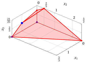
An optimal solution \({ \tilde{\boldsymbol x}}(\, LP \,)\) is:

\[ \tilde{x}_1=1,~~\tilde{x}_2=0,~~\tilde{x}_3=\dfrac{2}{5} \]

the optimal value \(z(\, LP \,)\) is \(\dfrac{34}{5}.\)

In violet the first and the second vertex explored by the previous execution of the revised simplex algorithm (before reaching the optimal one depicted in blue).

Exercise 11.19: Revised simplex algorithm (P46)

Consider the following LP problem in canonical maximization form with \(n=3\) variables and \(m=3\) constraints:

\[ \begin{array}{rrrrrrrr} {\max} & {5}\, {x_1} & {+} & {6}\, {x_2} & {+} & {10}\, {x_3} \\[2ex] \text{subject to} & {9}\, {x_1} & {+} & {2}\, {x_2} & {+} & {2}\, {x_3} & {\le} & {11} \\[2ex] & {2}\, {x_1} & {+} & {6}\, {x_2} & {+} & {6}\, {x_3} & {\le} & {16} \\[2ex] & {4}\, {x_1} & {+} & {2}\, {x_2} & {+} & {7}\, {x_3} & {\le} & {10} \\[2ex] & {x_1,} & & {x_2,} & & {x_3} & {\ge} & {0} \end{array} \]

By introducing the slack variables, we get the following LP problem in standard maximization form with \(n+m=6\) variables and \(m=3\) constraints:

\[ \begin{array}{rrcrcrcrcrcrcr} {\max} & {5}\, {x_1} & {+} & {6}\, {x_2} & {+} & {10}\, {x_3} \\[2ex] \text{subject to} & {9}\, {x_1} & {+} & {2}\, {x_2} & {+} & {2}\, {x_3} & {+} & {x_4} & & & & & {=} & {11} \\[2ex] & {2}\, {x_1} & {+} & {6}\, {x_2} & {+} & {6}\, {x_3} & & & {+} & {x_5} & & & {=} & {16} \\[2ex] & {4}\, {x_1} & {+} & {2}\, {x_2} & {+} & {7}\, {x_3} & & & & & {+} & {x_6} & {=} & {10} \\[2ex] & {x_1,} & & {x_2,} & & {x_3,} & & {x_4,} & & {x_5,} & & {x_6} & {\ge} & {0} \end{array} \]

Questions

• Execute the revised simplex algorithm to find an optimal solution of this LP problem using Bland's rule to select the pivot column and the pivot row.

Solution

We have:

\[ {\boldsymbol A}= \begin{pmatrix} 9 & 2 & 2 & 1 & 0 & 0\\ 2 & 6 & 6 & 0 & 1 & 0\\ 4 & 2 & 7 & 0 & 0 & 1 \end{pmatrix} \quad {\boldsymbol b}= \begin{pmatrix} 11\\ 16\\ 10 \end{pmatrix} \quad {\boldsymbol c}= \begin{pmatrix} 5\\ 6\\ 10\\ 0\\ 0\\ 0 \end{pmatrix} \quad {\boldsymbol x}= \begin{pmatrix} x_1 \\ x_2 \\ x_3 \\ x_4 \\ x_5 \\ x_6 \end{pmatrix} \]

• Initialization

  Since it is an LP problem in standard form obtained from an LP problem in canonical form with \(~{\boldsymbol b} \ge 0\) by adding the slack variables, the partition \(\pazocal{B}=\{4,5,6\}\) and \(\pazocal{N}=\{1,2,3\}\) is associated with the following basic feasible solution:

  \[ \begin{pmatrix} x_4 \\ x_5 \\ x_6 \end{pmatrix} = \begin{pmatrix} 11\\ 16\\ 10 \end{pmatrix} \text{ and } \begin{pmatrix} x_1 \\ x_2 \\ x_3 \end{pmatrix} = \begin{pmatrix} 0\\ 0\\ 0 \end{pmatrix} \]

• Iteration 1

  With \(\pazocal{B}= \{4,~~5,~~6\}\) and \(\pazocal{N}= \{1,~~2,~~3\}\), we have:

  \[ {\boldsymbol x}_{\pazocal{B}}= \begin{pmatrix} x_4 \\ x_5 \\ x_6 \end{pmatrix} ~~ {\boldsymbol A}_{\pazocal{B}}= \begin{pmatrix} 1 & 0 & 0\\ 0 & 1 & 0\\ 0 & 0 & 1 \end{pmatrix} ~~ {\boldsymbol c}_{\pazocal{B}}= \begin{pmatrix} 0\\ 0\\ 0 \end{pmatrix} ~~ {{ \bar{\boldsymbol b}}}= \begin{pmatrix} 11\\ 16\\ 10 \end{pmatrix} \]
  \[ {\boldsymbol x}_{\pazocal{N}}= \begin{pmatrix} x_1 \\ x_2 \\ x_3 \end{pmatrix} ~~ {\boldsymbol A}_{\pazocal{N}}= \begin{pmatrix} 9 & 2 & 2\\ 2 & 6 & 6\\ 4 & 2 & 7 \end{pmatrix} ~~ {\boldsymbol c}_{\pazocal{N}}= \begin{pmatrix} 5\\ 6\\ 10 \end{pmatrix} \]

  Optimality check

  We solve \({\boldsymbol \pi} \; {\boldsymbol A}_{\pazocal{B}} = {\boldsymbol c}'_{\pazocal{B}}\) to compute \({\boldsymbol \pi} = {{{\boldsymbol c}'_{\pazocal{B}} \; {\boldsymbol A}_{\pazocal{B}}^{-1}}}\), first system of linear equations:

  \[\begin{equation*} \begin{cases} \begin{array}{rrrrrrr} {\pi_4} & & & & & {=} & {0} \\[2ex] & & {\pi_5} & & & {=} & {0} \\[2ex] & & & & {\pi_6} & {=} & {0} \end{array} \end{cases} \qquad {\boldsymbol \pi}= \begin{pmatrix} 0 & 0 & 0\\ \end{pmatrix} \end{equation*}\]

  We compute the basic feasible solution value \({\bar{z}} = {\boldsymbol \pi} \; {\boldsymbol b} = \begin{pmatrix} 0 & 0 & 0\\ \end{pmatrix} \begin{pmatrix} 11\\ 16\\ 10 \end{pmatrix} = 0\)

  We compute the reduced costs \({{ \bar{\boldsymbol c}}'} = {{\boldsymbol c}'_{\pazocal{N}} - {\boldsymbol \pi} \; {\boldsymbol A}_{\pazocal{N}}}\):

  \[ \begin{aligned} {{ \bar{\boldsymbol c}}'} &= \begin{pmatrix} 5 & 6 & 10\\ \end{pmatrix} - \begin{pmatrix} 0 & 0 & 0\\ \end{pmatrix} \begin{pmatrix} 9 & 2 & 2\\ 2 & 6 & 6\\ 4 & 2 & 7 \end{pmatrix} \\[1ex] &= \underbrace{ \begin{pmatrix} 5 & 6 & 10\\ \end{pmatrix} }_{{c_{1}~~~c_{2}~~~c_{3}}} - \underbrace{ \begin{pmatrix} 0 & 0 & 0\\ \end{pmatrix} }_{{\boldsymbol \pi}\;{\boldsymbol A}_{1} ~~{\boldsymbol \pi}\;{\boldsymbol A}_{2} ~~{\boldsymbol \pi}\;{\boldsymbol A}_{3}} = \underbrace{ \begin{pmatrix} 5 & 6 & 10\\ \end{pmatrix} }_{{\bar{c}_{1}~~~\bar{c}_{2}~~~\bar{c}_{3}}} \end{aligned} \]

  Not all reduced costs are non-positive then we perform a pivoting operation.

  Pivoting operation

  Since \({c}_{1} > {\boldsymbol \pi} \;{\boldsymbol A}_{1}\), \(x_1\) is the pivot column and we have \({\boldsymbol A}_{1} = \begin{pmatrix} 9\\ 2\\ 4 \end{pmatrix}\)

  We solve \({\boldsymbol A}_{\pazocal{B}} \; {\boldsymbol d} = {\boldsymbol A}_{1}\) to compute \({\boldsymbol d}={ {\boldsymbol A}_{\pazocal{B}}^{-1}} {\boldsymbol A}_{1}\), second system of linear equations:

  \[\begin{equation*} \begin{cases} \begin{array}{rrrrrrr} {d_4} & & & & & {=} & {9} \\[2ex] & & {d_5} & & & {=} & {2} \\[2ex] & & & & {d_6} & {=} & {4} \end{array} \end{cases} \qquad {\boldsymbol d}= \begin{pmatrix} 9\\ 2\\ 4 \end{pmatrix} \end{equation*}\]

  We have to find the largest \(t\) such that \({{ \bar{\boldsymbol b}}} - t \; {{\boldsymbol d}} \ge 0\):

  \[ \begin{cases} \underbrace{11 -t \cdot 9\ge 0}_{x_4 \ge 0} \\[2ex] \underbrace{16 -t \cdot 2\ge 0}_{x_5 \ge 0} \\[2ex] \underbrace{10 -t \cdot 4\ge 0}_{x_6 \ge 0} \end{cases} \qquad \begin{cases} t\le \dfrac{11}{9} \\[2ex] t\le 8 \\[2ex] t\le \dfrac{5}{2} \end{cases} \text{ then } t_{m}=\dfrac{11}{9} \]

  Accordingly the value of the pivot column becomes \(t_{m}\), i.e., \(x_1=\dfrac{11}{9}\). The value of \(x_4\) becomes zero and \(x_4\) is the pivot row. The other basic variables take values \({ \bar{\boldsymbol b}} - t_{m} \; {\boldsymbol d}\), then we have:

  \[ \begin{aligned} x_5 &= 16 - \dfrac{11}{9} \cdot 2 = \dfrac{122}{9} \\[2ex] x_6 &= 10 - \dfrac{11}{9} \cdot 4 = \dfrac{46}{9} \end{aligned} \]

• Iteration 2

  With \(\pazocal{B}= \{1,~~5,~~6\}\) and \(\pazocal{N}= \{2,~~3,~~4\}\), we have:

  \[ {\boldsymbol x}_{\pazocal{B}}= \begin{pmatrix} x_1 \\ x_5 \\ x_6 \end{pmatrix} ~~ {\boldsymbol A}_{\pazocal{B}}= \begin{pmatrix} 9 & 0 & 0\\ 2 & 1 & 0\\ 4 & 0 & 1 \end{pmatrix} ~~ {\boldsymbol c}_{\pazocal{B}}= \begin{pmatrix} 5\\ 0\\ 0 \end{pmatrix} ~~ {{ \bar{\boldsymbol b}}}= \begin{pmatrix} \dfrac{11}{9}\\[2ex] \dfrac{122}{9}\\[2ex] \dfrac{46}{9} \end{pmatrix} \]
  \[ {\boldsymbol x}_{\pazocal{N}}= \begin{pmatrix} x_2 \\ x_3 \\ x_4 \end{pmatrix} ~~ {\boldsymbol A}_{\pazocal{N}}= \begin{pmatrix} 2 & 2 & 1\\ 6 & 6 & 0\\ 2 & 7 & 0 \end{pmatrix} ~~ {\boldsymbol c}_{\pazocal{N}}= \begin{pmatrix} 6\\ 10\\ 0 \end{pmatrix} \]

  Optimality check

  We solve \({\boldsymbol \pi} \; {\boldsymbol A}_{\pazocal{B}} = {\boldsymbol c}'_{\pazocal{B}}\) to compute \({\boldsymbol \pi} = {{{\boldsymbol c}'_{\pazocal{B}} \; {\boldsymbol A}_{\pazocal{B}}^{-1}}}\), first system of linear equations:

  \[\begin{equation*} \begin{cases} \begin{array}{rrrrrrr} {9}\, {\pi_1} & {+} & {2}\, {\pi_5} & {+} & {4}\, {\pi_6} & {=} & {5} \\[2ex] & & {\pi_5} & & & {=} & {0} \\[2ex] & & & & {\pi_6} & {=} & {0} \end{array} \end{cases} \qquad {\boldsymbol \pi}= \begin{pmatrix} \dfrac{5}{9} & 0 & 0\\ \end{pmatrix} \end{equation*}\]

  We compute the basic feasible solution value \({\bar{z}} = {\boldsymbol \pi} \; {\boldsymbol b} = \begin{pmatrix} \dfrac{5}{9} & 0 & 0\\ \end{pmatrix} \begin{pmatrix} 11\\ 16\\ 10 \end{pmatrix} = \dfrac{55}{9}\)

  We compute the reduced costs \({{ \bar{\boldsymbol c}}'} = {{\boldsymbol c}'_{\pazocal{N}} - {\boldsymbol \pi} \; {\boldsymbol A}_{\pazocal{N}}}\):

  \[ \begin{aligned} {{ \bar{\boldsymbol c}}'} &= \begin{pmatrix} 6 & 10 & 0\\ \end{pmatrix} - \begin{pmatrix} \dfrac{5}{9} & 0 & 0\\ \end{pmatrix} \begin{pmatrix} 2 & 2 & 1\\ 6 & 6 & 0\\ 2 & 7 & 0 \end{pmatrix} \\[1ex] &= \underbrace{ \begin{pmatrix} 6 & 10 & 0\\ \end{pmatrix} }_{{c_{2}~~~c_{3}~~~c_{4}}} - \underbrace{ \begin{pmatrix} \dfrac{10}{9} & \dfrac{10}{9} & \dfrac{5}{9}\\ \end{pmatrix} }_{{\boldsymbol \pi}\;{\boldsymbol A}_{2} ~~{\boldsymbol \pi}\;{\boldsymbol A}_{3} ~~{\boldsymbol \pi}\;{\boldsymbol A}_{4}} = \underbrace{ \begin{pmatrix} \dfrac{44}{9} & \dfrac{80}{9} & -\dfrac{5}{9}\\ \end{pmatrix} }_{{\bar{c}_{2}~~~\bar{c}_{3}~~~\bar{c}_{4}}} \end{aligned} \]

  Not all reduced costs are non-positive then we perform a pivoting operation.

  Pivoting operation

  Since \({c}_{2} > {\boldsymbol \pi} \;{\boldsymbol A}_{2}\), \(x_2\) is the pivot column and we have \({\boldsymbol A}_{2} = \begin{pmatrix} 2\\ 6\\ 2 \end{pmatrix}\)

  We solve \({\boldsymbol A}_{\pazocal{B}} \; {\boldsymbol d} = {\boldsymbol A}_{2}\) to compute \({\boldsymbol d}={ {\boldsymbol A}_{\pazocal{B}}^{-1}} {\boldsymbol A}_{2}\), second system of linear equations:

  \[\begin{equation*} \begin{cases} \begin{array}{rrrrrrr} {9}\, {d_1} & & & & & {=} & {2} \\[2ex] {2}\, {d_1} & {+} & {d_5} & & & {=} & {6} \\[2ex] {4}\, {d_1} & & & {+} & {d_6} & {=} & {2} \end{array} \end{cases} \qquad {\boldsymbol d}= \begin{pmatrix} \dfrac{2}{9}\\[2ex] \dfrac{50}{9}\\[2ex] \dfrac{10}{9} \end{pmatrix} \end{equation*}\]

  We have to find the largest \(t\) such that \({{ \bar{\boldsymbol b}}} - t \; {{\boldsymbol d}} \ge 0\):

  \[ \begin{cases} \underbrace{\dfrac{11}{9} -t \cdot \dfrac{2}{9}\ge 0}_{x_1 \ge 0} \\[2ex] \underbrace{\dfrac{122}{9} -t \cdot \dfrac{50}{9}\ge 0}_{x_5 \ge 0} \\[2ex] \underbrace{\dfrac{46}{9} -t \cdot \dfrac{10}{9}\ge 0}_{x_6 \ge 0} \end{cases} \qquad \begin{cases} t\le \dfrac{11}{2} \\[2ex] t\le \dfrac{61}{25} \\[2ex] t\le \dfrac{23}{5} \end{cases} \text{ then } t_{m}=\dfrac{61}{25} \]

  Accordingly the value of the pivot column becomes \(t_{m}\), i.e., \(x_2=\dfrac{61}{25}\). The value of \(x_5\) becomes zero and \(x_5\) is the pivot row. The other basic variables take values \({ \bar{\boldsymbol b}} - t_{m} \; {\boldsymbol d}\), then we have:

  \[ \begin{aligned} x_1 &= \dfrac{11}{9} - \dfrac{61}{25} \cdot \dfrac{2}{9} = \dfrac{17}{25} \\[2ex] x_6 &= \dfrac{46}{9} - \dfrac{61}{25} \cdot \dfrac{10}{9} = \dfrac{12}{5} \end{aligned} \]

• Iteration 3

  With \(\pazocal{B}= \{1,~~2,~~6\}\) and \(\pazocal{N}= \{3,~~4,~~5\}\), we have:

  \[ {\boldsymbol x}_{\pazocal{B}}= \begin{pmatrix} x_1 \\ x_2 \\ x_6 \end{pmatrix} ~~ {\boldsymbol A}_{\pazocal{B}}= \begin{pmatrix} 9 & 2 & 0\\ 2 & 6 & 0\\ 4 & 2 & 1 \end{pmatrix} ~~ {\boldsymbol c}_{\pazocal{B}}= \begin{pmatrix} 5\\ 6\\ 0 \end{pmatrix} ~~ {{ \bar{\boldsymbol b}}}= \begin{pmatrix} \dfrac{17}{25}\\[2ex] \dfrac{61}{25}\\[2ex] \dfrac{12}{5} \end{pmatrix} \]
  \[ {\boldsymbol x}_{\pazocal{N}}= \begin{pmatrix} x_3 \\ x_4 \\ x_5 \end{pmatrix} ~~ {\boldsymbol A}_{\pazocal{N}}= \begin{pmatrix} 2 & 1 & 0\\ 6 & 0 & 1\\ 7 & 0 & 0 \end{pmatrix} ~~ {\boldsymbol c}_{\pazocal{N}}= \begin{pmatrix} 10\\ 0\\ 0 \end{pmatrix} \]

  Optimality check

  We solve \({\boldsymbol \pi} \; {\boldsymbol A}_{\pazocal{B}} = {\boldsymbol c}'_{\pazocal{B}}\) to compute \({\boldsymbol \pi} = {{{\boldsymbol c}'_{\pazocal{B}} \; {\boldsymbol A}_{\pazocal{B}}^{-1}}}\), first system of linear equations:

  \[\begin{equation*} \begin{cases} \begin{array}{rrrrrrr} {9}\, {\pi_1} & {+} & {2}\, {\pi_2} & {+} & {4}\, {\pi_6} & {=} & {5} \\[2ex] {2}\, {\pi_1} & {+} & {6}\, {\pi_2} & {+} & {2}\, {\pi_6} & {=} & {6} \\[2ex] & & & & {\pi_6} & {=} & {0} \end{array} \end{cases} \qquad {\boldsymbol \pi}= \begin{pmatrix} \dfrac{9}{25} & \dfrac{22}{25} & 0\\ \end{pmatrix} \end{equation*}\]

  We compute the basic feasible solution value \({\bar{z}} = {\boldsymbol \pi} \; {\boldsymbol b} = \begin{pmatrix} \dfrac{9}{25} & \dfrac{22}{25} & 0\\ \end{pmatrix} \begin{pmatrix} 11\\ 16\\ 10 \end{pmatrix} = \dfrac{451}{25}\)

  We compute the reduced costs \({{ \bar{\boldsymbol c}}'} = {{\boldsymbol c}'_{\pazocal{N}} - {\boldsymbol \pi} \; {\boldsymbol A}_{\pazocal{N}}}\):

  \[ \begin{aligned} {{ \bar{\boldsymbol c}}'} &= \begin{pmatrix} 10 & 0 & 0\\ \end{pmatrix} - \begin{pmatrix} \dfrac{9}{25} & \dfrac{22}{25} & 0\\ \end{pmatrix} \begin{pmatrix} 2 & 1 & 0\\ 6 & 0 & 1\\ 7 & 0 & 0 \end{pmatrix} \\[1ex] &= \underbrace{ \begin{pmatrix} 10 & 0 & 0\\ \end{pmatrix} }_{{c_{3}~~~c_{4}~~~c_{5}}} - \underbrace{ \begin{pmatrix} 6 & \dfrac{9}{25} & \dfrac{22}{25}\\ \end{pmatrix} }_{{\boldsymbol \pi}\;{\boldsymbol A}_{3} ~~{\boldsymbol \pi}\;{\boldsymbol A}_{4} ~~{\boldsymbol \pi}\;{\boldsymbol A}_{5}} = \underbrace{ \begin{pmatrix} 4 & -\dfrac{9}{25} & -\dfrac{22}{25}\\ \end{pmatrix} }_{{\bar{c}_{3}~~~\bar{c}_{4}~~~\bar{c}_{5}}} \end{aligned} \]

  Not all reduced costs are non-positive then we perform a pivoting operation.

  Pivoting operation

  Since \({c}_{3} > {\boldsymbol \pi} \;{\boldsymbol A}_{3}\), \(x_3\) is the pivot column and we have \({\boldsymbol A}_{3} = \begin{pmatrix} 2\\ 6\\ 7 \end{pmatrix}\)

  We solve \({\boldsymbol A}_{\pazocal{B}} \; {\boldsymbol d} = {\boldsymbol A}_{3}\) to compute \({\boldsymbol d}={ {\boldsymbol A}_{\pazocal{B}}^{-1}} {\boldsymbol A}_{3}\), second system of linear equations:

  \[\begin{equation*} \begin{cases} \begin{array}{rrrrrrr} {9}\, {d_1} & {+} & {2}\, {d_2} & & & {=} & {2} \\[2ex] {2}\, {d_1} & {+} & {6}\, {d_2} & & & {=} & {6} \\[2ex] {4}\, {d_1} & {+} & {2}\, {d_2} & {+} & {d_6} & {=} & {7} \end{array} \end{cases} \qquad {\boldsymbol d}= \begin{pmatrix} 0\\ 1\\ 5 \end{pmatrix} \end{equation*}\]

  We have to find the largest \(t\) such that \({{ \bar{\boldsymbol b}}} - t \; {{\boldsymbol d}} \ge 0\):

  \[ \begin{cases} \underbrace{\dfrac{61}{25} -t \cdot 1\ge 0}_{x_2 \ge 0} \\[2ex] \underbrace{\dfrac{12}{5} -t \cdot 5\ge 0}_{x_6 \ge 0} \end{cases} \qquad \begin{cases} t\le \dfrac{61}{25} \\[2ex] t\le \dfrac{12}{25} \end{cases} \text{ then } t_{m}=\dfrac{12}{25} \]

  Accordingly the value of the pivot column becomes \(t_{m}\), i.e., \(x_3=\dfrac{12}{25}\). The value of \(x_6\) becomes zero and \(x_6\) is the pivot row. The other basic variables take values \({ \bar{\boldsymbol b}} - t_{m} \; {\boldsymbol d}\), then we have:

  \[ \begin{aligned} x_1 &= \dfrac{17}{25} - \dfrac{12}{25} \cdot 0 = \dfrac{17}{25} \\[2ex] x_2 &= \dfrac{61}{25} - \dfrac{12}{25} \cdot 1 = \dfrac{49}{25} \end{aligned} \]

• Iteration 4

  With \(\pazocal{B}= \{1,~~2,~~3\}\) and \(\pazocal{N}= \{4,~~5,~~6\}\), we have:

  \[ {\boldsymbol x}_{\pazocal{B}}= \begin{pmatrix} x_1 \\ x_2 \\ x_3 \end{pmatrix} ~~ {\boldsymbol A}_{\pazocal{B}}= \begin{pmatrix} 9 & 2 & 2\\ 2 & 6 & 6\\ 4 & 2 & 7 \end{pmatrix} ~~ {\boldsymbol c}_{\pazocal{B}}= \begin{pmatrix} 5\\ 6\\ 10 \end{pmatrix} ~~ {{ \bar{\boldsymbol b}}}= \begin{pmatrix} \dfrac{17}{25}\\[2ex] \dfrac{49}{25}\\[2ex] \dfrac{12}{25} \end{pmatrix} \]
  \[ {\boldsymbol x}_{\pazocal{N}}= \begin{pmatrix} x_4 \\ x_5 \\ x_6 \end{pmatrix} ~~ {\boldsymbol A}_{\pazocal{N}}= \begin{pmatrix} 1 & 0 & 0\\ 0 & 1 & 0\\ 0 & 0 & 1 \end{pmatrix} ~~ {\boldsymbol c}_{\pazocal{N}}= \begin{pmatrix} 0\\ 0\\ 0 \end{pmatrix} \]

  Optimality check

  We solve \({\boldsymbol \pi} \; {\boldsymbol A}_{\pazocal{B}} = {\boldsymbol c}'_{\pazocal{B}}\) to compute \({\boldsymbol \pi} = {{{\boldsymbol c}'_{\pazocal{B}} \; {\boldsymbol A}_{\pazocal{B}}^{-1}}}\), first system of linear equations:

  \[\begin{equation*} \begin{cases} \begin{array}{rrrrrrr} {9}\, {\pi_1} & {+} & {2}\, {\pi_2} & {+} & {4}\, {\pi_3} & {=} & {5} \\[2ex] {2}\, {\pi_1} & {+} & {6}\, {\pi_2} & {+} & {2}\, {\pi_3} & {=} & {6} \\[2ex] {2}\, {\pi_1} & {+} & {6}\, {\pi_2} & {+} & {7}\, {\pi_3} & {=} & {10} \end{array} \end{cases} \qquad {\boldsymbol \pi}= \begin{pmatrix} \dfrac{1}{25} & \dfrac{18}{25} & \dfrac{4}{5}\\ \end{pmatrix} \end{equation*}\]

  We compute the basic feasible solution value \({\bar{z}} = {\boldsymbol \pi} \; {\boldsymbol b} = \begin{pmatrix} \dfrac{1}{25} & \dfrac{18}{25} & \dfrac{4}{5}\\ \end{pmatrix} \begin{pmatrix} 11\\ 16\\ 10 \end{pmatrix} = \dfrac{499}{25}\)

  We compute the reduced costs \({{ \bar{\boldsymbol c}}'} = {{\boldsymbol c}'_{\pazocal{N}} - {\boldsymbol \pi} \; {\boldsymbol A}_{\pazocal{N}}}\):

  \[ \begin{aligned} {{ \bar{\boldsymbol c}}'} &= \begin{pmatrix} 0 & 0 & 0\\ \end{pmatrix} - \begin{pmatrix} \dfrac{1}{25} & \dfrac{18}{25} & \dfrac{4}{5}\\ \end{pmatrix} \begin{pmatrix} 1 & 0 & 0\\ 0 & 1 & 0\\ 0 & 0 & 1 \end{pmatrix} \\[1ex] &= \underbrace{ \begin{pmatrix} 0 & 0 & 0\\ \end{pmatrix} }_{{c_{4}~~~c_{5}~~~c_{6}}} - \underbrace{ \begin{pmatrix} \dfrac{1}{25} & \dfrac{18}{25} & \dfrac{4}{5}\\ \end{pmatrix} }_{{\boldsymbol \pi}\;{\boldsymbol A}_{4} ~~{\boldsymbol \pi}\;{\boldsymbol A}_{5} ~~{\boldsymbol \pi}\;{\boldsymbol A}_{6}} = \underbrace{ \begin{pmatrix} -\dfrac{1}{25} & -\dfrac{18}{25} & -\dfrac{4}{5}\\ \end{pmatrix} }_{{\bar{c}_{4}~~~\bar{c}_{5}~~~\bar{c}_{6}}} \end{aligned} \]

  All reduced costs are non-positive, then the basic feasible solution

  \[ {\boldsymbol x}_{\pazocal{B}}= \begin{pmatrix} x_1 \\ x_2 \\ x_3 \end{pmatrix}=\begin{pmatrix} \dfrac{17}{25}\\[2ex] \dfrac{49}{25}\\[2ex] \dfrac{12}{25} \end{pmatrix} \text{ and } {\boldsymbol x}_{\pazocal{N}}= \begin{pmatrix} x_4 \\ x_5 \\ x_6 \end{pmatrix}=\begin{pmatrix} 0\\ 0\\ 0 \end{pmatrix} \]

  is an optimal solution of the LP problem and \({\bar{z}} = \dfrac{499}{25}\) is the optimal solution value.

Graphical solution:

The feasible region of the LP problem (in canonical form) is the polyhedron shaded in red:

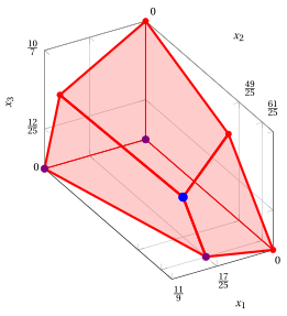
An optimal solution \({ \tilde{\boldsymbol x}}(\, LP \,)\) is:

\[ \tilde{x}_1=\dfrac{17}{25},~~\tilde{x}_2=\dfrac{49}{25},~~\tilde{x}_3=\dfrac{12}{25} \]

the optimal value \(z(\, LP \,)\) is \(\dfrac{499}{25}.\)

In violet the first, the second and the third vertex explored by the previous execution of the revised simplex algorithm (before reaching the optimal one depicted in blue).