Integer linear programming

Part 1 · Models and bounds · Chapter 1 · Lecture notes, volume 1 (PDF) · Exercises: Integer linear programming

Prerequisites

• From the module Linear Programming: Chapter 2 «Half-spaces and polyhedra» and Chapter 4 «Linear Programming problems» (the canonical maximization form, the feasible region, optimal solutions and the optimal value), and Chapter 5 «Possible outcomes and equivalent formulations» (infeasible, unbounded and optimal problems).

Objectives

At the end of this chapter you will be able to:

• write an ILP problem in canonical maximization form, and distinguish ILP, BIP and MIP problems;

• draw the feasible region of a small ILP problem and find an optimal solution graphically;

• explain why the feasible region is not convex, and what the three outcomes of an ILP problem are;

• explain why complete enumeration fails, and how much it costs;

• say why bounds on the optimal value are needed to avoid enumeration.

1.1 Canonical maximization form

Definition 1.1: Integer Linear Programming problems in canonical maximization form

Given:

1. an objective-function vector \(\vet c \in \Z^{n}\)

2. a constraint matrix \(\mat A \in \Z^{m \times n}\)

3. a right-hand-side (RHS) vector \(\vet b \in \Z^{m}\) with \(m\) rows

   \[ \underbrace{ \begin{pmatrix} c_{1} \\ c_{2} \\ \vdots \\ c_{n} \\ \end{pmatrix} }_{\vet c} \in \Z^{n} \qquad \qquad \underbrace{ \begin{pmatrix} a_{11} & a_{12} & \dots & a_{1n}\\ a_{21} & a_{22} & \dots & a_{2n}\\ \vdots & \vdots & \ddots & \vdots \\ a_{m1} & a_{m2} & \dots & a_{mn}\\ \end{pmatrix} }_{\mat A} \in \Z^{m \times n} \qquad \qquad \underbrace{ \begin{pmatrix} b_{1} \\ b_{2} \\ \vdots \\ b_{m} \\ \end{pmatrix} }_{\vet b} \in \Z^{m} \]

an Integer Linear Programming problem ILP in canonical maximization form with \(n\) non-negative integer variables

\[ \underbrace{ \begin{pmatrix} x_{1} \\ x_{2} \\ \vdots \\ x_{n} \\ \end{pmatrix} }_{\vet x} \in \Z^{n}_{\ge 0} \]

and \(m\) less-than-or-equal-to linear constraints is the following optimization problem:

\[\begin{align*} \label{ObjFunc} && \max \;\; \underbrace{\sum_{j =1}^n c_j \, x_j}_{\vet c\T \vet x} \qquad \qquad \qquad \qquad \qquad \qquad \tag{1.1a}\\[1ex] \label{Cons} && \text{subject to} \quad \underbrace{\sum_{j =1}^n a_{ij} \, x_j \le b_i, \qquad \forall i \in \{1,2,\dots,m\}}_{\mat A\,\vet x \le \vet b}, \tag{1.1b}\\[1ex] \label{integrality}&& \underbrace{x_j \in \Z_{\ge 0}, \qquad \forall j \in \{1,2,\dots,n\}}_{\vet x \in \Z^n_{\ge 0}}. \tag{1.1c} \end{align*}\]

• The data \(\vet c\), \(\mat A\) and \(\vet b\) are integer, as in the whole module.

• With a slight abuse of notation, we write the ILP problem (1.1) in compact form as

  \[ \max \big\{\, \vet c\T \vet x ~:~ \mat A\,\vet x \le \vet b,~ \vet x \in \Z^n_{\ge 0} \,\big\}. \]

• The set \(\Z^n\) of the points of \(\R^n\) with integer components is called the integer lattice.

An ILP problem (1.1) is an LP problem in canonical maximization form with the additional requirement \(\vet x \in \Z^n\): the linear function \(\vet c\T \vet x\) is maximized over the points of the integer lattice that satisfy the constraints.

• If all the variables are restricted to \(\{0,1\}\), the problem is a binary integer linear programming (BIP) problem. If only some of the variables are integer, the problem is a mixed integer linear programming (MIP) problem.

• Constraints \(\ge\) and \(=\), and minimization problems, are brought to the canonical maximization form as in linear programming.

Example 1.1: ILP problem in canonical maximization form

Consider the following input data of an ILP problem with \(n=2\) and \(m=2\):

\[ \vet c= \begin{pmatrix} 3 \\[1ex] 2\\ \end{pmatrix} \qquad \mat A= \begin{pmatrix} 10 & 4 \\[1ex] 4 & 14 \\ \end{pmatrix} \qquad \vet b= \begin{pmatrix} 45 \\[1ex] 49\\ \end{pmatrix} \]

The numerical entries of the two column vectors and the matrix are

\[ c_1=3,~c_2=2,~a_{11}=10,~a_{12}=4,~a_{21}=4,~a_{22}=14,~b_1=45,~b_2=49. \]

The associated ILP problem in canonical maximization form with \(n=2\) non-negative integer variables and \(m=2\) less-than-or-equal-to linear constraints reads as follows:

\[ \begin{array}{rrrrrrr} {\max} & {3}\, {x_1} & {+} & {2}\, {x_2} \\[1ex] \text{subject to} & {10}\, {x_1} & {+} & {4}\, {x_2} & {\le} & {45} \\[1ex] & {4}\, {x_1} & {+} & {14}\, {x_2} & {\le} & {49} \\[1ex] & {x_1,} & & {x_2} & {\in} & {\Z_{\ge 0}} \end{array} \]

The variables \(x_1\) and \(x_2\) can be read as the numbers of cars of two types to produce: this ILP problem is the car example, the guiding example of the module.

1.1.1 Feasible region and objective function

Definition 1.2: feasible region and objective function

• The feasible region of an ILP problem (1.1) is the set \(F\) defined as follows:

  \[\begin{equation*} \label{FeasibleRegion} \begin{split} F = \left\{~ \underbrace{ \begin{pmatrix} x_{1} \\ x_{2} \\ \vdots \\ x_{n} \\ \end{pmatrix}}_{\vet x} \in \Z^n : \right. ~~ & \underbrace{\sum_{j=1}^n a_{ij} \, x_j \le b_i,~~\forall i \in \{1,2,\dots,m\}}_{\mat A\,\vet x \le \vet b}, \\[1ex] & \left. \vphantom{\begin{pmatrix} x_{1} \\ x_{2} \\ \vdots \\ x_{n} \end{pmatrix}} \underbrace{x_j \ge 0,~~\forall j \in \{1,2,\dots,n\}}_{\vet x \ge \vet 0} ~\right\}. \end{split} \tag{1.2} \end{equation*}\]

• The objective function \(\eqref{ObjFunc}\) of an ILP problem (1.1) to be maximized is the (scalar) linear function \(f\) defined as follows:

  \[\begin{equation*} \label{ObjectiveFunction} f: \Z^{n} \rightarrow \R, \qquad f : \underbrace{\begin{pmatrix} x_1 \\ x_2 \\ \vdots \\ x_n \end{pmatrix}}_{\vet x} \mapsto \underbrace{\sum_{j=1}^n c_j x_j}_{\vet c\T \vet x} \tag{1.3} \end{equation*}\]

• Let \(P = \{\, \vet x \in \R^n : \mat A\,\vet x \le \vet b,~ \vet x \ge \vet 0 \,\}\) be the polyhedron of the constraints, that is, the feasible region of the LP problem with the same data. The feasible region of the ILP problem is

  \[ F = P \cap \Z^n. \]

• The set \(F\) is made of isolated points of the lattice, hence it is not convex.

Example 1.2: feasible region

Consider the ILP problem of Example 1.1. The feasible region \(F\) is the set of the \(16\) black points of the following figure, the points of the lattice \(\Z^2\) in the polyhedron \(P\) (red).

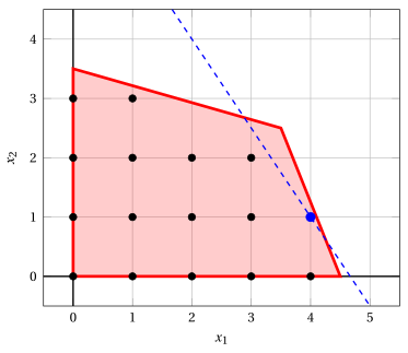
The car example: the feasible region of the ILP problem is the set of its \(16\) integer points (black) inside the polyhedron (red). The optimal solution \((4,1)\) is blue, with the objective line \(3\,x_1 + 2\,x_2 = 14\) (dashed).

The point \(\bar{\vet x} = (2,2)\) belongs to \(F\), because \(10 \cdot 2 + 4 \cdot 2 = 28 \le 45\) and \(4 \cdot 2 + 14 \cdot 2 = 36 \le 49\). The point \((4,2)\) does not belong to \(F\), because \(10 \cdot 4 + 4 \cdot 2 = 48 > 45\). The point \((\frac{7}{2},\frac{5}{2})\) belongs to \(P\) but not to \(F\), because it is not integer.

1.1.2 Optimal solution and optimal value

Definition 1.3: optimal solution and optimal value

• A point \(\tilde{\vet x}(\ILP) \in F\) is an optimal solution of the ILP problem (1.1) if

  \[ \tilde{\vet x}(\ILP) \in \argmax \big\{\, \vet c\T \vet x ~:~ \vet x \in F \,\big\}. \]

• The value

  \[ z(\ILP) = \underbrace{\max \big\{\, \vet c\T \vet x ~:~ \vet x \in F \,\big\}}_{=\vet c\T \tilde{\vet x}(\ILP)} \]

  is the optimal value of the ILP problem (1.1).

• A point \(\bar{\vet x} \in F\) is a feasible solution of the ILP problem. An optimal solution is a feasible solution with the largest value of the objective function.

The goal of an ILP problem (1.1) is to find an optimal solution \(\tilde{\vet x}(\ILP)\), whenever it exists, rather than merely determining the optimal value \(z(\ILP)\).

1.1.3 Graphical solution method

An optimal solution of an ILP problem (1.1) with two variables can be graphically determined by moving the level line of the objective function in the direction of its gradient, until the last point of the lattice in the polyhedron \(P\) is reached.

Example 1.3: Graphical solution method

Consider the ILP problem of Example 1.1. The gradient of the objective function is \(\nabla f = (3,2)\). Moving the level line \(3\,x_1 + 2\,x_2 = z\) in the direction of \(\nabla f\), the last point of \(F\) reached is \((4,1)\), on the dashed line \(3\,x_1 + 2\,x_2 = 14\) of the figure of Example 1.2. No other point of \(F\) lies on this line.

The car example has the unique optimal solution \(\tilde{\vet x}(\ILP) = (4,1)\), with optimal value \(z(\ILP) = 14\).

1.2 Possible outcomes

• As in linear programming, an ILP problem has exactly one of three outcomes: it is infeasible (\(F = \emptyset\)), unbounded (the objective function is not bounded from above on \(F\)) or it has an optimal solution.

• If the polyhedron \(P\) is bounded, then \(F\) is a finite set, and an optimal solution exists as soon as \(F \neq \emptyset\).

Example 1.4: an infeasible ILP problem with a feasible LP problem

The ILP problem

\[ \max \big\{\, x_1 ~:~ 2\,x_1 \le 1,~ -2\,x_1 \le -1,~ x_1 \in \Z_{\ge 0} \,\big\} \]

is infeasible, because the constraints require \(x_1 = \frac{1}{2}\). The LP problem with the same data is feasible, with the unique feasible solution \(x_1 = \frac{1}{2}\).

Example 1.5: an unbounded ILP problem

The ILP problem

\[ \max \big\{\, x_1 + x_2 ~:~ x_1 - x_2 \le 1,~ x_1, x_2 \in \Z_{\ge 0} \,\big\} \]

is unbounded: the points \((k,k)\), \(k \in \Z_{\ge 0}\), are feasible, with value \(2k\).

1.3 Complete enumeration

• When the feasible region is a finite set we can find an optimal solution by complete enumeration: we compute the objective function for every feasible solution and keep the best. For the car example, there are \(16\) points:

\[ \begin{array}{ccc|ccc} \hline {x_1} & {x_2} & {z} & {x_1} & {x_2} & {z} \\ \hline {0} & {0} & {0} & {3} & {1} & {11} \\ {1} & {0} & {3} & {\mathbf{4}} & {\mathbf{1}} & {\mathbf{14}} \\ {2} & {0} & {6} & {0} & {2} & {4} \\ {3} & {0} & {9} & {1} & {2} & {7} \\ {4} & {0} & {12} & {2} & {2} & {10} \\ {0} & {1} & {2} & {3} & {2} & {13} \\ {1} & {1} & {5} & {0} & {3} & {6} \\ {2} & {1} & {8} & {1} & {3} & {9} \\ \hline \end{array} \]

• The best value is \(14\), in \((4,1)\) (in bold). Here the method works, because the model is tiny.

• Consider now the simplest case, \(n\) binary variables and no other constraint. Every variable takes \(2\) values, so there are \(2^n\) solutions: the vertices of an \(n\)-dimensional hypercube.

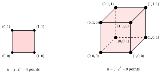
The solutions of \(n\) binary variables without other constraints: the \(2^n\) vertices of an \(n\)-dimensional hypercube, for \(n=2\) (a square) and \(n=3\) (a cube).

• The number \(2^n\) explodes. With \(n = 80\) variables there are about \(1.2 \cdot 10^{24}\) solutions, comparable to the estimated number of stars in the universe, and with \(n = 266\) variables about \(1.2 \cdot 10^{80}\), comparable to the estimated number of atoms in the observable universe.

• Suppose that a computer examines \(10^{9}\) solutions per second, and then a computer \(1000\) times faster, \(10^{12}\) solutions per second. The time needed to enumerate \(2^n\) solutions is:

\(n\)	\(2^n\)	at \(10^{9}\) solutions/s	at \(10^{12}\) solutions/s
20	\(\approx 1.05 \cdot 10^{6}\)	\(\approx 1.05\,\mathrm{ms}\)	\(\approx 1.05\,\mu\mathrm{s}\)
30	\(\approx 1.07 \cdot 10^{9}\)	\(\approx 1.07\,\mathrm{s}\)	\(\approx 1.07\,\mathrm{ms}\)
40	\(\approx 1.10 \cdot 10^{12}\)	\(\approx 18.3\,\mathrm{min}\)	\(\approx 1.10\,\mathrm{s}\)
50	\(\approx 1.13 \cdot 10^{15}\)	\(\approx 13.0\,\mathrm{days}\)	\(\approx 18.8\,\mathrm{min}\)
60	\(\approx 1.15 \cdot 10^{18}\)	\(\approx 36.5\,\mathrm{years}\)	\(\approx 13.3\,\mathrm{days}\)
70	\(\approx 1.18 \cdot 10^{21}\)	\(\approx 374\,\mathrm{centuries}\)	\(\approx 37.4\,\mathrm{years}\)
80	\(\approx 1.21 \cdot 10^{24}\)	\(\approx 3.8 \cdot 10^{5}\,\mathrm{centuries}\)	\(\approx 383\,\mathrm{centuries}\)

Complete enumeration is impractical already for models of moderate size. A computer \(1000\) times faster gains only about \(10\) variables, because \(2^{10} = 1024 \approx 1000\).

• The way out is to avoid enumerating. If we know a lower bound and an upper bound on the optimal value, we can exclude entire regions of feasible solutions without visiting them. The two bounds come from two different sources, the feasible solutions and the relaxations: they are the subject of the next chapter, «Primal and dual bounds».

1.4 Typical mistakes

Warning

• Believing that the feasible region is convex. It is the set of the integer points of a polyhedron, not the polyhedron. The midpoint of two feasible solutions can be infeasible.

• Believing that the feasible region is always finite. It is finite only if the polyhedron is bounded; otherwise the ILP problem can be unbounded.

• Believing that a feasible LP problem gives a feasible ILP problem. The LP problem can have solutions while no integer point satisfies the constraints.

• Taking a good feasible solution as optimal. Without a bound from the other side (next chapter) there is no certificate of optimality.

1.5 In summary

In summary

• An ILP problem maximizes a linear function over the integer points of a polyhedron; its feasible region is not convex, and it is finite when the polyhedron is bounded.

• The outcomes are infeasible, unbounded or optimal, and a feasible LP problem can have an infeasible ILP version.

• Complete enumeration costs \(2^n\) evaluations for \(n\) binary variables: it is not an option beyond very small models.

• To avoid enumeration we need bounds on \(z(\ILP)\) from both sides: feasible solutions and relaxations, the subject of the next chapter.

Dashboard of the car example. No bounds yet: the next chapter gives the first lower and upper bounds.

---

Exercises on this chapter: Integer linear programming