Primal and dual bounds¶

Part 1 · Models and bounds · Chapter 2 · Lecture notes, volume 1 (PDF) · Exercises: Primal and dual bounds · App: Integer points and the LP relaxation

Prerequisites

From this module, the chapter «Integer linear programming»: ILP problems, feasible and optimal solutions, complete enumeration, and the car example.
From the module Linear Programming, Chapter 9 «Duality theory»: the dual problem, weak duality and strong duality.
From the same module, Chapter 6 «Simplex algorithm»: an LP problem that has an optimal solution has an optimal vertex.

Objectives

At the end of this chapter you will be able to:

obtain a primal bound (a lower bound) on the optimal value from a feasible solution, also with a simple heuristic algorithm;
build the LP relaxation of an ILP problem and use its optimal value as a dual bound (an upper bound), rounded down when it is valid;
compute the optimality gap from a primal bound and a dual bound;
explain why rounding an optimal LP solution gives a feasible solution at best;
derive upper bounds on the variables from the constraints, and say when they help;
obtain a dual bound from non-negative multipliers of the constraints, and recognize the dual problem as the problem of the best multipliers.

Where we were

In the previous chapter we saw that complete enumeration is not an option, and that we need bounds on the optimal value from both sides. We now obtain them: primal bounds from feasible solutions, and dual bounds from relaxations.

2.1 Primal and dual bounds¶

Definition 2.1: primal bound, dual bound and optimality gap

Consider an ILP problem in canonical maximization form, with feasible region \(F\) and optimal value \(z(\ILP)\).

Given a feasible solution \(\bar{\vet x} \in F\), its value \(\LB(\bar{\vet x}) = \sum_{j=1}^n c_j \, \bar{x}_j\) is a primal bound on \(z(\ILP)\).
A value \(\UB\) such that \(\sum_{j=1}^n c_j \, x_j \le \UB\) for every \(\vet x \in F\) is a dual bound on \(z(\ILP)\).
Given a primal bound \(\LB \ne 0\) and a dual bound \(\UB\), the optimality gap is

\[\begin{equation*} \label{gap} \text{optimality gap} = \frac{\UB - \LB}{|\LB|} . \tag{2.1} \end{equation*}\]

In a maximization problem the primal bounds are lower bounds and the dual bounds are upper bounds. A primal bound comes from one feasible solution; a dual bound is a statement on all the feasible solutions at once.

For every feasible solution \(\bar{\vet x}\) and every dual bound \(\UB\):

\[ \LB(\bar{\vet x}) ~\le~ z(\ILP) ~\le~ \UB . \]

A feasible solution is certified optimal when the optimality gap is zero.

Definition 2.2: relaxation

Given an ILP problem \(\max \{ \vet c\T \vet x : \vet x \in F \}\), the problem \(\max \{ \vet c\T \vet x : \vet x \in R \}\) is a relaxation of the ILP problem if \(F \subseteq R\). We denote its optimal value by \(z(R)\).

A maximization over a larger region cannot give a smaller value: the optimal value of a relaxation is a dual bound, \(z(\ILP) \le z(R)\).

2.2 Primal bounds: heuristic solutions¶

Definition 2.3: heuristic algorithm

A heuristic algorithm is a method that finds feasible solutions quickly, with no guarantee of optimality. The value of every solution it finds is a primal bound.

A good feasible solution is a good primal bound.

Example 2.1: primal bound

For the feasible solution \((2,2)\) of the car example we get \(\LB = 3 \cdot 2 + 2 \cdot 2 = 10\), so \(z(\ILP) \ge 10\).

Definition 2.4: of integer part of a number

Given \(y \in \R\), the integer part of \(y\) is \(\lfloor y \rfloor = \max \{ q \in \Z : q \le y \}\).

Example 2.2: two heuristic algorithms for the car example

The one-variable heuristic sets a single variable to its maximum value, with the other one equal to \(0\), and keeps the better of the two solutions.
1. Only \(x_1\) (\(x_2 = 0\)): \(\bar{x}_1 = \min\{\lfloor \frac{45}{10} \rfloor, \lfloor \frac{49}{4} \rfloor\} = \min\{4, 12\} = 4\), so \(\bar{\vet x} = (4,0)\) and \(\LB = 12\).
2. Only \(x_2\) (\(x_1 = 0\)): \(\bar{x}_2 = \min\{\lfloor \frac{45}{4} \rfloor, \lfloor \frac{49}{14} \rfloor\} = \min\{11, 3\} = 3\), so \(\bar{\vet x} = (0,3)\) and \(\LB = 6\).
The two-step heuristic sets first one variable to its maximum value, and then the other one to its maximum value with the residual right-hand sides. It keeps the better of the two solutions.
1. \(x_1\) first: \(\bar{x}_1 = 4\) uses \(40\) and \(16\), leaving \(5\) and \(33\). Then \(\bar{x}_2 = \min\{\lfloor \frac{5}{4} \rfloor, \lfloor \frac{33}{14} \rfloor\} = \min\{1, 2\} = 1\), so \(\bar{\vet x} = (4,1)\) and \(\LB = 14\).
2. \(x_2\) first: \(\bar{x}_2 = 3\) uses \(12\) and \(42\), leaving \(33\) and \(7\). Then \(\bar{x}_1 = \min\{\lfloor \frac{33}{10} \rfloor, \lfloor \frac{7}{4} \rfloor\} = \min\{3, 1\} = 1\), so \(\bar{\vet x} = (1,3)\) and \(\LB = 9\).

Heuristic	Order	\(\bar{x}_1\)	\(\bar{x}_2\)	\(\LB\)
one-variable	\(x_1\)	\(4\)	\(0\)	\(12\)
one-variable	\(x_2\)	\(0\)	\(3\)	\(6\)
two-step	\(x_1\) first	\(4\)	\(1\)	\(14\)
two-step	\(x_2\) first	\(1\)	\(3\)	\(9\)

The two-step heuristic gives a better primal bound, but it needs more computation. This trade-off between the quality of the solution and the computational effort is typical of heuristic algorithms.
Here the best primal bound is \(\LB = 14\), in \((4,1)\). A primal bound alone is not a certificate of optimality: a dual bound is needed.

2.3 The LP relaxation¶

Definition 2.5: LP relaxation

The linear programming (LP) relaxation of an ILP problem in canonical maximization form is the LP problem obtained by replacing the integrality constraints \(x_j \in \Z_{\ge 0}\) with the non-negativity constraints \(x_j \ge 0\), for all \(j \in \{1,2,\dots,n\}\):

\[\begin{align*} && \max \;\;{\sum_{j =1}^n c_j \, x_j} \label{ObjFunc_LP} \tag{2.2a}\\[2ex] && \text{subject to} \quad {\sum_{j =1}^n a_{ij} \, x_j} &\leq b_i, & \forall i \in \{1,2,\dots,m\}, \label{Cons_LP} \tag{2.2b}\\[2ex] &&x_j &\ge 0, & \forall j \in \{1,2,\dots,n\}. \label{non_negativity_LP} \tag{2.2c} \end{align*}\]

We denote by \(z(\LP)\) the optimal value of the LP relaxation, and by \(\tilde{\vet x}(\LP)\) an optimal solution. We always write the argument, because in the same example \(\tilde{\vet x}(\ILP)\) and \(\tilde{\vet x}(\LP)\) are different points.

Proposition 2.6: upper bound from the LP relaxation

Every feasible solution of the ILP problem is feasible for its LP relaxation, hence

\[\begin{equation*} z(\ILP) \le z(\LP). \label{LP_BOUND} \tag{2.3} \end{equation*}\]

Moreover, if an optimal solution of the LP relaxation is integer, then it is an optimal solution of the ILP problem.

Proof

The feasible region \(F\) of the ILP problem is contained in the polyhedron of the LP relaxation, and the objective function is the same. The maximum over a larger set is not smaller than the maximum over a subset. If \(\tilde{\vet x}(\LP)\) is integer, it belongs to \(F\) and has value \(z(\LP) \ge z(\ILP)\): it is optimal for the ILP problem. □

The value of a feasible solution can be an integer, and it is at most \(z(\LP)\): then it is at most the largest integer not exceeding \(z(\LP)\).

Observation 2.7: rounding the upper bound

If all the variables are integer and all the costs \(c_j\) are integer, then

\[\begin{equation*} z(\ILP) \le \lfloor z(\LP) \rfloor. \label{LP_BOUND_2} \tag{2.4} \end{equation*}\]

In all the other cases the bound \(\lfloor z(\LP) \rfloor\) is not valid.

In this module all the ILP problems have integer data, so the bound \(\eqref{LP_BOUND_2}\) always holds. In a MIP problem with a continuous variable the value of a feasible solution is not necessarily an integer, and the bound cannot be rounded.

Example 2.3: the LP relaxation of the car example

The LP relaxation of the car example has the optimal solution

\[ \tilde{x}_1 = \frac{7}{2}, \quad \tilde{x}_2 = \frac{5}{2}, \qquad z(\LP) = \frac{31}{2}, \]

and it is fractional: it is not feasible for the ILP problem.
Since the costs are integer, we have the upper bound \(\lfloor z(\LP) \rfloor = 15\). Together with the primal bound \(14\) of the feasible solution \((4,1)\) of Example 2.2:

\[ 14 ~\le~ z(\ILP) ~\le~ 15. \]

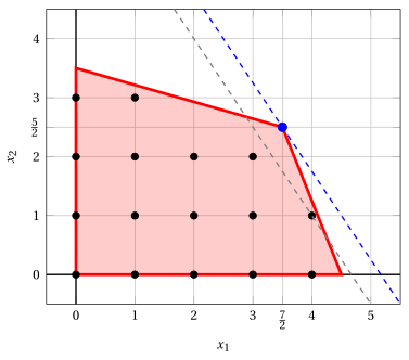
The LP relaxation of the car example: the feasible region (red), its \(16\) integer points (black) and the optimal solution \((\frac{7}{2},\frac{5}{2})\) of the LP relaxation (blue), with the objective line \(3\,x_1 + 2\,x_2 = \frac{31}{2}\) through it (dashed). The gray dashed line is the objective line of the optimal ILP solution.

The optimal value is \(14\) or \(15\). With \(\UB = 15\) and \(\LB = 14\) the optimality gap \(\eqref{gap}\) is \(\frac{1}{14} \approx 7.1\%\): the solution \((4,1)\) is not yet certified optimal.

2.4 Rounding the solution of the LP relaxation¶

Feasible ILP solutions can typically be obtained by rounding an optimal solution of the LP relaxation. But no rounding technique guarantees to find an optimal ILP solution.

Example 2.4: rounding in the car example

The optimal solution of the LP relaxation is \(\tilde{\vet x}(\LP) = (\frac{7}{2},\frac{5}{2})\). Rounding to the nearest integer gives \((4,3)\), which is infeasible: \(10 \cdot 4 + 4 \cdot 3 = 52 > 45\).
Rounding down both components gives the feasible solution \(\bar{\vet x} = (3,2)\), with \(\LB = 3 \cdot 3 + 2 \cdot 2 = 13\). The optimal ILP solution is \(\tilde{\vet x}(\ILP) = (4,1)\), with \(z(\ILP) = 14\): rounding does not give the optimum, and the bounds are \(13 \le z(\ILP) \le 15\).

Example 2.5: rounding works, but the bound is not tight

Consider the following ILP problem; its LP relaxation has \(x_1, x_2 \ge 0\) instead of the integrality constraints:

\[ \begin{array}{rrrrrrr} {\max} & {2}\, {x_1} & {+} & {4}\, {x_2} \\[1ex] \text{subject to} & {-}\, {x_1} & {+} & \, {x_2} & {\le} & {2} \\[1ex] & {8}\, {x_1} & {+} & {2}\, {x_2} & {\le} & {19} \\[1ex] & {x_1,} & & {x_2} & {\in} & {\Z_{\ge 0}} \end{array} \]

The optimal solution of the LP relaxation is \(\tilde{\vet x}(\LP) = (\frac{3}{2},\frac{7}{2})\), with \(z(\LP) = 17\) and \(\lfloor z(\LP) \rfloor = 17\), so \(z(\ILP) \le 17\).
Rounding down both components we get the feasible solution \(\bar{\vet x} = (\lfloor \frac{3}{2} \rfloor, \lfloor \frac{7}{2} \rfloor) = (1,3)\), with \(\LB = 2 \cdot 1 + 4 \cdot 3 = 14\).
The optimal ILP solution is \(\tilde{\vet x}(\ILP) = (1,3)\), with \(z(\ILP) = 14\): the rounded solution is optimal. But the bounds \(14 \le z(\ILP) \le 17\) do not prove it.

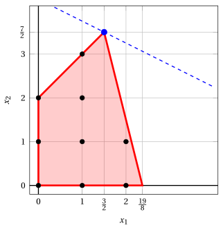
The second example: the feasible region of the LP relaxation (red), the integer points (black) and the optimal solution of the LP relaxation (blue), with the objective line \(2\,x_1 + 4\,x_2 = 17\) (dashed).

Example 2.6: rounding fails

Consider the following ILP problem:

\[ \begin{array}{rrrrrrr} {\max} & {25}\, {x_1} & {+} & {16}\, {x_2} \\[1ex] \text{subject to} & {50}\, {x_1} & {+} & {31}\, {x_2} & {\le} & {250} \\[1ex] & {-3}\, {x_1} & {+} & {2}\, {x_2} & {\le} & {4} \\[1ex] & {x_1,} & & {x_2} & {\in} & {\Z_{\ge 0}} \end{array} \]

The optimal solution of the LP relaxation is \(\tilde{\vet x}(\LP) = (\frac{376}{193}, \frac{950}{193}) \approx (1.94, 4.92)\), with \(z(\LP) = \frac{24600}{193} \approx 127.46\). Hence \(z(\ILP) \le \lfloor z(\LP) \rfloor = 127\).
Rounding to the nearest integer gives \((2,5)\), which is infeasible: \(50 \cdot 2 + 31 \cdot 5 = 255 > 250\). Rounding \(\tilde{x}_1\) up and \(\tilde{x}_2\) down gives the feasible solution \(\bar{\vet x} = (2,4)\), with \(\LB = 25 \cdot 2 + 16 \cdot 4 = 114\).
The optimal ILP solution is \(\tilde{\vet x}(\ILP) = (5,0)\), with \(z(\ILP) = 125\). It is far from \(\tilde{\vet x}(\LP)\), and no rounding of \(\tilde{\vet x}(\LP)\) finds it.

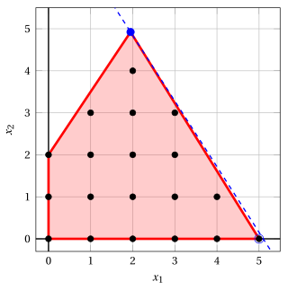
The third example: the integer points (black) are far from the optimal solution \((\frac{376}{193},\frac{950}{193})\) of the LP relaxation (blue). The optimal ILP solution is \((5,0)\) (blue circle). The dashed line is the objective line \(25\,x_1 + 16\,x_2 = \frac{24600}{193}\).

Optimal ILP solutions can be quite far from optimal solutions of the LP relaxation. The value of the LP relaxation, instead, is often a good bound: here \(125 \le z(\LP) \approx 127.46\).

2.5 Upper bounds on the variables¶

Proposition 2.8: upper bounds on the variables

Let \(\sum_{j=1}^n a_{ij} \, x_j \le b_i\) be a constraint with \(a_{ij} \ge 0\) for all \(j\). Then every feasible solution of the ILP problem satisfies

\[\begin{equation*} \label{vub} x_j \le \left\lfloor \frac{b_i}{a_{ij}} \right\rfloor, \qquad \forall j \text{ such that } a_{ij} > 0. \tag{2.5} \end{equation*}\]

Proof

Since all the variables are non-negative and all the coefficients are non-negative, \(a_{ij} \, x_j \le \sum_{k=1}^n a_{ik} \, x_k \le b_i\), so \(x_j \le \frac{b_i}{a_{ij}}\). The variable is integer, so it does not exceed the integer part of \(\frac{b_i}{a_{ij}}\). □

If several constraints give a bound on \(x_j\), we keep the smallest. The bounds cut off parts of the polyhedron of the LP relaxation, and no integer point.

The upper bounds on the variables improve the LP relaxation only if they cut off its optimal solution.

Example 2.7: upper bounds on the variables of the car example

Both constraints of the car example have non-negative coefficients:

\[\begin{align*} x_1 &\le \min \left\{ \left\lfloor \tfrac{45}{10} \right\rfloor, \left\lfloor \tfrac{49}{4} \right\rfloor \right\} = \min\{4, 12\} = 4,\\ x_2 &\le \min \left\{ \left\lfloor \tfrac{45}{4} \right\rfloor, \left\lfloor \tfrac{49}{14} \right\rfloor \right\} = \min\{11, 3\} = 3. \end{align*}\]

The inequalities \(x_1 \le 4\) and \(x_2 \le 3\) are satisfied by all the integer points of the car example, and they can be added to the model. They cut off two regions of the polyhedron, and no integer point.

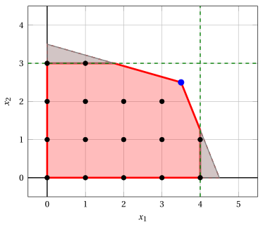
The variable upper bounds \(x_1 \le 4\) and \(x_2 \le 3\) (green) cut off the two gray regions of the LP relaxation (red) and no integer point. The optimal solution of the LP relaxation (blue) is not cut off.

The optimal solution of the LP relaxation, \((\frac{7}{2},\frac{5}{2})\), satisfies both inequalities. It is not cut off, so the optimal value of the LP relaxation does not change, and the upper bound is still \(15\).

Example 2.8: upper bounds that cut off the LP optimum

Consider the objective function \(x_1 - x_2\) on the constraints of the car example, whose optimal ILP solution is \((4,0)\) with \(z(\ILP) = 4\). Before the bounds, the optimal solution of the LP relaxation is \((\frac{9}{2},0)\) with \(z(\LP) = \frac{9}{2}\); after \(x_1 \le 4\) it is \((4,0)\) with \(z(\LP) = 4\), which is integer and therefore optimal.

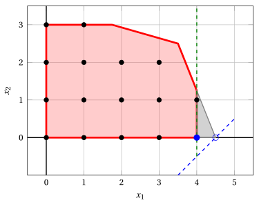
The objective \(x_1 - x_2\): the variable upper bound \(x_1 \le 4\) (green) cuts off the gray triangle and the optimal solution \((\frac{9}{2},0)\) of the LP relaxation (blue circle). The new optimal solution \((4,0)\) (blue) is integer. The dashed line is \(x_1 - x_2 = \frac{9}{2}\).

The value of the LP relaxation improves from \(\frac{9}{2}\) to \(4\). The rounded bound \(\lfloor \frac{9}{2} \rfloor = 4\) was already \(4\): a better formulation does not always improve the rounded bound.

2.6 Dual bounds¶

A dual bound can also be obtained without solving the LP relaxation, by combining the constraints with non-negative multipliers \(\pi_i\), one for each constraint.

Definition 2.9: dual problem of the LP relaxation

The dual problem D(LP) of the LP relaxation (2.2) is the following LP problem, with optimal value \(z(\mathrm{D(LP)})\):

\[\begin{align*} && \min \;\;{\sum_{i =1}^m b_i \, \pi_i} \label{ObjFunc_D} \tag{2.6a}\\[2ex] && \text{subject to} \quad {\sum_{i =1}^m a_{ij} \, \pi_i} &\geq c_j, & \forall j \in \{1,2,\dots,n\}, \label{Cons_D} \tag{2.6b}\\[2ex] &&\pi_i &\ge 0, & \forall i \in \{1,2,\dots,m\}. \label{non_negativity_D} \tag{2.6c} \end{align*}\]

Multiplying the constraint \(i\) by \(\pi_i \ge 0\) and summing, we get an inequality whose coefficients are at least the costs, by \(\eqref{Cons_D}\). The multipliers must be non-negative: a negative multiplier would reverse the inequality.

Proposition 2.10: dual bounds

For every feasible solution \(\bar{\vet \pi}\) of the dual problem (2.6),

\[ z(\ILP) ~\le~ z(\LP) ~\le~ \sum_{i=1}^m b_i \, \bar{\pi}_i . \]

By strong duality, \(z(\mathrm{D(LP)}) = z(\LP)\): the best multipliers give exactly the value of the LP relaxation.

Proof

Let \(\vet x\) be feasible for the LP relaxation. Multiplying the constraint \(i\) by \(\bar{\pi}_i \ge 0\) and summing, \(\sum_{j=1}^n \big( \sum_{i=1}^m a_{ij} \, \bar{\pi}_i \big) x_j \le \sum_{i=1}^m b_i \, \bar{\pi}_i\). By \(\eqref{Cons_D}\) and \(x_j \ge 0\), the left-hand side is at least \(\sum_{j=1}^n c_j \, x_j\). Hence \(\sum_{j=1}^n c_j \, x_j \le \sum_{i=1}^m b_i \, \bar{\pi}_i\) for every feasible \(\vet x\). □

Every feasible solution of the dual problem is a certificate of an upper bound, found without solving the LP relaxation. The best certificate is an optimal dual solution, and it has the same value as the LP relaxation.

Example 2.9: multipliers for the car example

A feasible solution of the LP relaxation does not give a dual bound: its value is neither a lower bound nor an upper bound on \(z(\ILP)\).

\((x_1, x_2)\)	feasible for the LP relaxation	integer	\(3\,x_1 + 2\,x_2\)
\((4, \frac{5}{4})\)	yes	no	\(\frac{29}{2} > 14\)
\((2, \frac{5}{2})\)	yes	no	\(11 < 14\)

Multiplying the first constraint of the car example by \(\frac{3}{4}\) we get

\[ \frac{15}{2}\,x_1 + 3\,x_2 \le \frac{135}{4}. \]

Since \(x_1, x_2 \ge 0\) and the coefficients \(\frac{15}{2}\) and \(3\) are at least the costs \(3\) and \(2\), we have \(3\,x_1 + 2\,x_2 \le \frac{15}{2}\,x_1 + 3\,x_2 \le \frac{135}{4}\): an upper bound of \(\frac{135}{4}\).
With multipliers \(\pi_1, \pi_2 \ge 0\) of the two constraints, the coefficients of the sum must be at least the costs:

\[\begin{align*} (10\,\pi_1 + 4\,\pi_2)\,x_1 + (4\,\pi_1 + 14\,\pi_2)\,x_2 &\le 45\,\pi_1 + 49\,\pi_2,\\ 10\,\pi_1 + 4\,\pi_2 \ge 3, \qquad 4\,\pi_1 + 14\,\pi_2 &\ge 2. \end{align*}\]

\((\pi_1, \pi_2)\)	valid multipliers	upper bound \(45\,\pi_1 + 49\,\pi_2\)
\((\frac{3}{4}, 0)\)	yes	\(\frac{135}{4}\)
\((0, \frac{3}{4})\)	yes	\(\frac{147}{4}\)
\((\frac{1}{5}, \frac{1}{4})\)	yes	\(\frac{85}{4}\)
\((\frac{1}{2}, 0)\)	yes	\(\frac{45}{2}\)
\((\frac{1}{5}, 0)\)	no: \(10 \cdot \frac{1}{5} = 2 < 3\)	–

The best multipliers, with the smallest value \(45\,\pi_1 + 49\,\pi_2\), solve the dual problem (2.6) of the car example:

\[ \begin{array}{rrrrrrr} {\min} & {45}\, {\pi_1} & {+} & {49}\, {\pi_2} \\[1ex] \text{subject to} & {10}\, {\pi_1} & {+} & {4}\, {\pi_2} & {\ge} & {3} \\[1ex] & {4}\, {\pi_1} & {+} & {14}\, {\pi_2} & {\ge} & {2} \\[1ex] & {\pi_1,} & & {\pi_2} & {\ge} & {0} \end{array} \]

Example 2.10: optimal dual solution of the car example

The optimal solution of the dual problem of Example 2.9 is \(\tilde{\vet \pi}(\mathrm{D(LP)}) = (\frac{17}{62},\frac{2}{31})\), and

\[ z(\mathrm{D(LP)}) = 45 \cdot \frac{17}{62} + 49 \cdot \frac{2}{31} = \frac{765}{62} + \frac{98}{31} = \frac{31}{2} = z(\LP). \]

The other two vertices of the dual feasible region give the bounds \(\frac{45}{2}\) and \(\frac{147}{4}\).

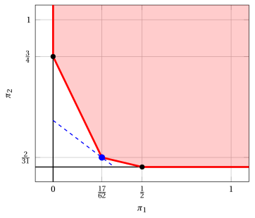
The feasible region of the dual LP problem (red, unbounded) and its optimal solution \((\frac{17}{62},\frac{2}{31})\) (blue), with the objective line \(45\,\pi_1 + 49\,\pi_2 = \frac{31}{2}\) (dashed). The other vertices (black) give the bounds \(\frac{45}{2}\) and \(\frac{147}{4}\).

2.6.1 Summary of the notation¶

ILP problem: optimal solution \(\tilde{\vet x}(\ILP)\), optimal value \(z(\ILP)\).
Primal bound: feasible solution \(\bar{\vet x}\) with \(\LB(\bar{\vet x}) = \sum_{j} c_j \, \bar{x}_j \le z(\ILP)\).
LP relaxation: optimal solution \(\tilde{\vet x}(\LP)\), optimal value \(z(\LP)\), upper bound \(z(\ILP) \le z(\LP)\).
Dual problem: optimal solution \(\tilde{\vet \pi}(\mathrm{D(LP)})\), optimal value \(z(\mathrm{D(LP)}) = z(\LP)\), and \(z(\ILP) \le \sum_i b_i \, \bar{\pi}_i\) for every dual feasible \(\bar{\vet \pi}\).

2.7 Typical mistakes¶

Warning

Taking a heuristic solution as optimal. A feasible solution gives only a primal bound. Without a dual bound with the same value there is no certificate of optimality.
Rounding the bound when it is not valid. The bound \(\lfloor z(\LP) \rfloor\) requires all the variables and all the costs to be integer. In a MIP problem the bound is \(z(\LP)\).
Rounding the solution and calling it optimal. A rounded solution is feasible at best, and in general not optimal. It may even be infeasible, as the nearest integer point \((2,5)\) of Example 2.6.
Using the value of a feasible LP solution as a bound. Only the optimal value of the LP relaxation, or the value of a dual feasible solution, is an upper bound.
Multipliers with a negative sign. The multipliers of constraints \(\le\) must be non-negative, and the combined coefficients must be at least the costs.
Deriving a bound on a variable from a constraint with negative coefficients. The proof of \(\eqref{vub}\) needs all the coefficients to be non-negative.
Believing that a stronger formulation always improves the bound. The bounds \(x_1 \le 4\) and \(x_2 \le 3\) leave the bound \(15\) of the car example unchanged.

2.8 In summary¶

In summary

Every feasible solution is a primal bound (a lower bound) on \(z(\ILP)\), and heuristic algorithms find good feasible solutions quickly.
The LP relaxation drops integrality, so \(z(\ILP) \le z(\LP)\); with integer variables and integer costs this dual bound (an upper bound) can be rounded down to \(\lfloor z(\LP) \rfloor\).
Primal and dual bound define the optimality gap; optimality is certified when the gap is zero.
Rounding an optimal LP solution gives a feasible solution at best, never a certificate.
The upper bounds on the variables \(x_j \le \lfloor b_i / a_{ij} \rfloor\) come from constraints with non-negative coefficients, and they help only if they cut off the LP optimum.
Non-negative multipliers of the constraints give dual bounds; the best ones solve the dual problem, whose optimal value is \(z(\LP)\).

Dashboard of the car example. The bounds on \(z(\ILP)\) found so far in this module (primal bound: lower; dual bound: upper):

Chapter	Lower bound	Upper bound	From
Primal and dual bounds	\(14\)	\(15\)	heuristic solution \((4, 1)\), and \(\lfloor z(\LP) \rfloor\) with \(z(\LP) = \tfrac{31}{2}\)

Exercises on this chapter: Primal and dual bounds

Interactive lab¶

The ideas of the chapter, hands on: move the sliders and drag the points. Each app also opens full page in the interactive lab: Integer points and the LP relaxation.