Optimization problems
Part 2 · Optimization problems · Chapter 5 · Lecture notes, volume 2 (PDF) · Slides · Exercises: Optimization problems · App: Optimum on an interval · App: Local and global optima
5.1 Optimization problems
Definition 5.1: optimization problem in minimization and maximization form
Given a set \(F \subseteq \mathbb{R}^n\) and a function \(f : D \subseteq \mathbb{R}^n \to \mathbb{R}\), with \(F \subseteq D\), the associated optimization problem \(P\) consists of:
-
in the minimization form, finding a point \(\tilde{\boldsymbol{x}}(P) \in F\) such that
\[ f(\tilde{\boldsymbol{x}}(P)) \le f(\boldsymbol{x}), \qquad \forall \boldsymbol{x} \in F; \] -
in the maximization form, finding a point \(\tilde{\boldsymbol{x}}(P) \in F\) such that
\[ f(\tilde{\boldsymbol{x}}(P)) \ge f(\boldsymbol{x}), \qquad \forall \boldsymbol{x} \in F. \]
5.1.1 Feasible region and objective function
-
The set \(F\) is called the feasible region of the optimization problem; its points \(\boldsymbol{x} \in F\) are called the feasible solutions of the optimization problem.
-
The function \(f\) is the objective function of the optimization problem; it assigns an objective value to each feasible solution.
Definition 5.2: optimal solution and optimal value
-
A point \(\tilde{\boldsymbol{x}}(P) \in F\) is called an optimal solution of the optimization problem.
-
In the minimization form,
\[ \tilde{\boldsymbol{x}}(P) \in \argmin \{\, f(\boldsymbol{x}) \;\text{subject to}\; \boldsymbol{x} \in F \,\}. \] -
In the maximization form,
\[ \tilde{\boldsymbol{x}}(P) \in \argmax \{\, f(\boldsymbol{x}) \;\text{subject to}\; \boldsymbol{x} \in F \,\}. \]
-
-
The value \(f(\tilde{\boldsymbol{x}}(P))\) is called the optimal value of the optimization problem, and it is denoted by \(z(P)\).
-
In the minimization form,
\[ z(P) = \underbrace{\min \{\, f(\boldsymbol{x}) \;\text{subject to}\; \boldsymbol{x} \in F \,\}}_{ =f(\tilde{\boldsymbol{x}}(P))}. \] -
In the maximization form,
\[ z(P) = \underbrace{\max \{\, f(\boldsymbol{x}) \;\text{subject to}\; \boldsymbol{x} \in F \,\}}_{ =f(\tilde{\boldsymbol{x}}(P))}. \]
-
-
An optimization problem may admit multiple (possibly infinitely many) optimal solutions, or none at all. In such cases, the operators \(\argmin\) and \(\argmax\) return the full set of optimal solutions when they exist, and return the empty set otherwise.
-
With a slight abuse of notation:
-
In the minimization form, we write the optimization problem as
\[ \min \{\, f(\boldsymbol{x}) \;\text{subject to}\; \boldsymbol{x} \in F \,\}. \] -
In the maximization form, we write the optimization problem as
\[ \max \{\, f(\boldsymbol{x}) \;\text{subject to}\; \boldsymbol{x} \in F \,\}. \]
Although we use the symbols “\(\min\)” and “\(\max\)”, the goal of an optimization problem is to find an optimal solution \(\tilde{\boldsymbol{x}}(P)\), whenever it exists, rather than merely determining the optimal value \(z(P)\).
-
-
In the figures of this chapter, the graph of the objective function over the feasible region is red, the feasible region is the red part of the \(x\)-axis and the optimal solutions are blue. An empty circle marks an endpoint that does not belong to the feasible region.
Example 5.1: an optimization problem with a quadratic objective function
Consider the following objective function and feasible region:
The associated optimization problems in minimization and maximization forms are:
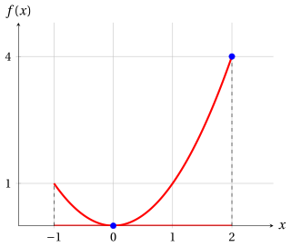
-
For the minimization form, since \(f(x) = x^2 \ge 0 = f(0)\) for every feasible \(x\), and \(x^2 = 0\) only for \(x=0\), the unique optimal solution and the optimal value are:
\[ \tilde{\boldsymbol x}(P) = (0) \quad \text{and} \quad z(P) = 0. \] -
For the maximization form, for every feasible \(x\) we have \(|x| \le 2\) and then \(f(x) = |x|^2 \le 4 = f(2)\), with \(x^2 = 4\) only for \(x=-2\) and \(x=2\); since \(-2 \notin F\), the unique optimal solution and the optimal value are:
\[ \tilde{\boldsymbol x}(P) = (2) \quad \text{and} \quad z(P) = 4. \]
The optimal solutions are found directly from the definition: we compare the value of the objective function at a candidate point with its value at every feasible solution.
Example 5.2: an optimization problem with infinitely many optimal solutions
Consider the following objective function and feasible region:
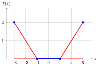
The objective function is \(f(x) = 0\) for \(-1 \le x \le 1\) and \(f(x) = |x|-1\) otherwise: its graph is made of three segments.
-
For the minimization form, \(f(x) \ge 0\) for every feasible \(x\), and \(f(x) = 0\) exactly for \(-1 \le x \le 1\). The problem has infinitely many optimal solutions (the blue segment) and the optimal value is:
\[ \argmin \big\{\, \max\{0,|x|-1\} \ \text{ subject to } -3 \le x \le 3 \,\big\} = [-1,1] \quad \text{and} \quad z(P) = 0. \] -
For the maximization form, for every feasible \(x\) we have \(|x| \le 3\) and then \(f(x) \le \max\{0,\, 3-1\} = 2\), with \(f(x) = 2\) only for \(x=-3\) and \(x=3\). The problem has two optimal solutions and the optimal value is:
\[ \argmax \big\{\, \max\{0,|x|-1\} \ \text{ subject to } -3 \le x \le 3 \,\big\} = \{-3,\,3\} \quad \text{and} \quad z(P) = 2. \]
-
An optimal solution of an optimization problem may not exist for one of the following three reasons:
-
If the objective function decreases indefinitely in a minimization problem or increases indefinitely in a maximization problem, the optimization problem is said to be unbounded. In these cases, \(z(P) = -\infty\) and \(z(P) = +\infty\), respectively.
-
If the feasible region is empty, meaning that no solutions exist, the optimization problem is said to be infeasible. In these cases, \(z(P)\) is not defined.
-
If the infimum (or supremum) of the objective function exists but is not attained within the feasible region, the optimization problem is said to have an unattainable infimum (or supremum), as in Examples 5.5 and Example 5.6. In these cases, \(z(P)\) is not defined.
-
-
In the minimization form, an optimal solution is a point of minimum, and the corresponding optimal value is the minimum of the objective function over the feasible region.
Similarly, in the maximization form, an optimal solution is a point of maximum, and the corresponding optimal value is the maximum of the objective function over the feasible region.
Example 5.3: an unbounded optimization problem
Consider the following objective function and feasible region:
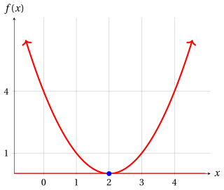
The feasible region is the whole real line: the graph continues upward on both sides of the figure.
-
For the minimization form, since \(f(x) = (x-2)^2 \ge 0 = f(2)\) for every \(x \in \R\), and \((x-2)^2 = 0\) only for \(x=2\), the unique optimal solution and the optimal value are:
\[ \tilde{\boldsymbol x}(P) = (2) \quad \text{and} \quad z(P) = 0. \] -
For the maximization form, the objective function increases indefinitely: for every value \(M \ge 0\), the feasible solution \(x = M+3\) has
\[ f(M+3) = (M+1)^2 \ge M+1 > M. \]No feasible solution can be optimal and the problem is unbounded: \(z(P) = +\infty\).
Example 5.4: an infeasible optimization problem
Consider the following objective function and feasible region:
Since \(x^2 \ge 0 > -1\) for every \(x \in \R\), no point satisfies the constraint and the feasible region is empty: \(F = \emptyset\). Both the minimization and the maximization form are infeasible: they have no feasible solution, hence no optimal solution, and \(z(P)\) is not defined.
Example 5.5: an optimization problem with an unattainable infimum
Consider the following objective function and feasible region:
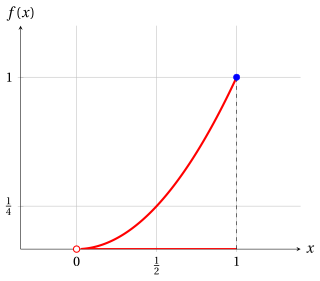
The point \(x=0\) does not belong to the feasible region (empty circle in the figure).
-
For the minimization form, \(f(x) = x^2 > 0\) for every feasible \(x\), and the values of \(f\) get as close to \(0\) as we want: the infimum of \(f\) over \(F\) is \(0\). However, no feasible solution is optimal: for every \(x \in F\), the point \(\frac{x}{2}\) is feasible and
\[ f\Big(\frac{x}{2}\Big) = \frac{x^2}{4} < x^2 = f(x). \]The problem has an unattainable infimum: there is no optimal solution and \(z(P)\) is not defined.
-
For the maximization form, for every feasible \(x\) we have \(0 < x \le 1\) and then \(f(x) = x^2 \le 1 = f(1)\), with \(x^2 = 1\) only for \(x=1\) in \(F\). The unique optimal solution and the optimal value are:
\[ \tilde{\boldsymbol x}(P) = (1) \quad \text{and} \quad z(P) = 1. \]
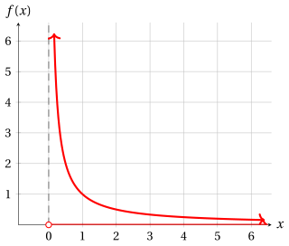
Example 5.6: an unattainable infimum at infinity
Consider the following objective function and feasible region:
The associated optimization problems in minimization and maximization forms are:
The point \(x=0\) does not belong to the feasible region (empty circle in the figure). The graph continues on the right, approaching the \(x\)-axis, and upward, approaching the dashed line \(x=0\).
-
For the minimization form, \(f(x) = \frac{1}{x} > 0\) for every feasible \(x\), and the values of \(f\) get as close to \(0\) as we want as \(x \to +\infty\): the infimum of \(f\) over \(F\) is \(0\). However, no feasible solution is optimal: for every \(x \in F\), the point \(2x\) is feasible and
\[ f(2x) = \frac{1}{2x} < \frac{1}{x} = f(x). \]The problem has an unattainable infimum: there is no optimal solution and
\[ \inf \bigg\{\, \frac{1}{x} \ \text{ subject to } x > 0 \,\bigg\} = 0, \qquad z(P) \ \text{is not defined}. \] -
For the maximization form, the objective function increases indefinitely as \(x \to 0^+\): for every value \(M > 0\), the feasible solution \(x = \frac{1}{M+1}\) has
\[ f\Big(\frac{1}{M+1}\Big) = M+1 > M. \]No feasible solution can be optimal and the problem is unbounded:
\[ \sup \bigg\{\, \frac{1}{x} \ \text{ subject to } x > 0 \,\bigg\} = +\infty \qquad \text{and} \qquad z(P) = +\infty. \]
5.1.2 Feasible solutions and bounds on the optimal value
-
Given
\[ \underbrace{ \begin{pmatrix} \bar x_1 \\ \bar x_2 \\ \vdots \\ \bar x_n \end{pmatrix} }_{\bar{\boldsymbol x}(P)} \in F \]a feasible solution of an optimization problem, we have
-
in minimization form, the following upper bound:
\[ z(P) \le \underbrace{f(\bar{\boldsymbol{x}}(P))}_{UB(\bar{\boldsymbol x})} . \] -
in maximization form, the following lower bound:
\[ \underbrace{f(\bar{\boldsymbol{x}}(P))}_{LB(\bar{\boldsymbol x})} \le z(P) . \]
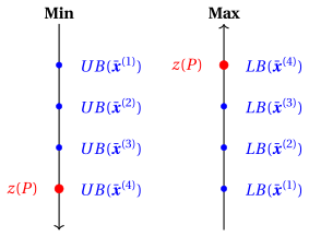
As an illustrative example, the figure below considers four feasible solutions
\[ \bar{\boldsymbol x}^{(1)}, \bar{\boldsymbol x}^{(2)}, \bar{\boldsymbol x}^{(3)}, \bar{\boldsymbol x}^{(4)} \in F \]and shows how they provide lower bounds in the maximization case and upper bounds in the minimization case for the optimal value \(z(P)\) (the fourth one attains the optimal value).
-
Example 5.7: bounds from feasible solutions
Consider again the objective function \(f(x) = x^2\) and the feasible region \(F=[-1,2]\) of the example with a quadratic objective function, where \(z(P) = 0\) in minimization form and \(z(P) = 4\) in maximization form. The feasible solutions
have objective values \(1\), \(\frac{1}{4}\) and \(1\). Therefore:
-
in minimization form, they give the upper bounds \(UB(\bar{\boldsymbol x}^{(1)}) = 1\), \(UB(\bar{\boldsymbol x}^{(2)}) = \frac{1}{4}\) and \(UB(\bar{\boldsymbol x}^{(3)}) = 1\) on \(z(P) = 0\); the best one is \(\frac{1}{4}\), the smallest;
-
in maximization form, they give the lower bounds \(LB(\bar{\boldsymbol x}^{(1)}) = 1\), \(LB(\bar{\boldsymbol x}^{(2)}) = \frac{1}{4}\) and \(LB(\bar{\boldsymbol x}^{(3)}) = 1\) on \(z(P) = 4\); the best one is \(1\), the largest.
None of these bounds is equal to the optimal value: a bound tells us how far the optimal value can be from the value of a known feasible solution, without computing it.
5.2 Properties of optimization problems
-
The following properties hold for every optimization problem.
-
In the following, we state properties using \(\min\) and \(\max\) only in the case where the minimum and maximum exist (i.e., they are attained on the feasible region); otherwise, the analogous statements hold by replacing \(\min/\max\) with \(\inf/\sup\).
-
For every objective function \(f\) and every feasible region \(F\), we have:
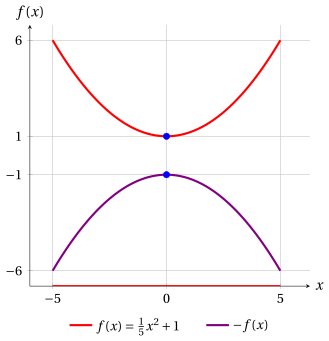
\[\begin{align*} \label{PropMinMax} \min \bigg\{\, f(\boldsymbol{x}) \text{ subject to } \boldsymbol{x}\in F \,\bigg\} &= -\,\max \bigg\{\, -f(\boldsymbol{x}) \text{ subject to } \boldsymbol{x}\in F \,\bigg\} \tag{5.1} \end{align*}\] -
The optimal solutions do not change: a point minimizes \(f\) over \(F\) if and only if it maximizes \(-f\) over \(F\). In the figures of this section, the original objective function is red, the transformed one is violet, the feasible region is the red part of the \(x\)-axis and the optimal solutions are blue.
Example 5.8: property: minimum and maximum
Indeed, \(\frac{1}{5}x^2+1 \ge 1\) and \(-\left(\frac{1}{5}x^2+1\right) \le -1\) for every \(x\), with equality only for \(x=0\): both optima are attained at \(x=0\).
-
For every objective function, every feasible region, and every \(a \in \R\), we have:
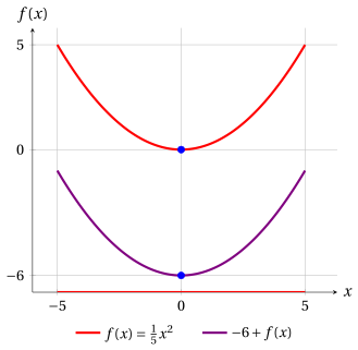
\[\begin{align*} \min \bigg\{\, a + f(\boldsymbol{x}) \text{ subject to } \boldsymbol{x}\in F \,\bigg\} &= a + \min \bigg\{\, f(\boldsymbol{x}) \text{ subject to } \boldsymbol{x}\in F \,\bigg\} \tag{5.2} \end{align*}\] -
Adding a constant moves the graph of the objective function up or down: the optimal solutions do not change.
Example 5.9: property: constant addition
Both minima are attained at \(x=0\), since \(\frac{1}{5}x^2 \ge 0\) for every \(x\), with equality only for \(x=0\).
-
For every objective function, every feasible region, and every \(a \in \R_{>0}\), we have:
\[\begin{align*} \min \bigg\{\, a\, f(\boldsymbol{x}) \text{ subject to } \boldsymbol{x}\in F \,\bigg\} &= a \; \min \bigg\{\, f(\boldsymbol{x}) \text{ subject to } \boldsymbol{x}\in F \,\bigg\} \tag{5.3} \end{align*}\] -
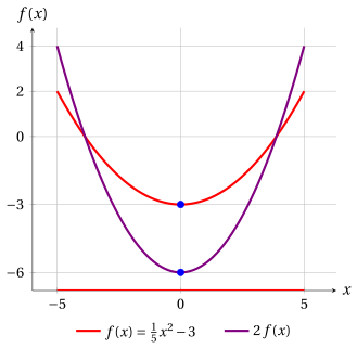
Multiplying by a positive constant stretches (or compresses) the graph vertically: the optimal solutions do not change.
Example 5.10: property: multiplication by a positive constant
Both minima are attained at \(x=0\), since \(\frac{1}{5}x^2-3 \ge -3\) for every \(x\), with equality only for \(x=0\).
-
For every objective function, every feasible region, and every \(a \in \R_{<0}\), we have:
\[\begin{align*} \min \bigg\{\, a\, f(\boldsymbol{x}) \text{ subject to } \boldsymbol{x}\in F \,\bigg\} &= a \; \max \bigg\{\, f(\boldsymbol{x}) \text{ subject to } \boldsymbol{x}\in F \,\bigg\} \tag{5.4} \end{align*}\] -
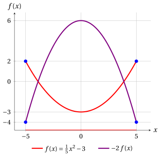
Multiplying by a negative constant turns the graph upside down: the points of minimum of \(a\,f\) are the points of maximum of \(f\).
Example 5.11: property: multiplication by a negative constant
For every feasible \(x\) we have \(|x| \le 5\) and then \(\frac{1}{5}x^2-3 \le \frac{25}{5}-3 = 2\), with equality only for \(x=-5\) and \(x=5\): both problems have the two optimal solutions \(x=-5\) and \(x=5\).
5.3 Local and global optimal solutions
Definition 5.3: point of minimum/maximum and minimum/maximum
Given a function \(f:D\subseteq \R^n \rightarrow \R\), a point \(\tilde{\boldsymbol x} \in D\) is
-
a point of minimum (global minimum point) of \(f\) in \(D\) if
\[\begin{equation*} f(\tilde{\boldsymbol x}) ~\le~ f({\boldsymbol x}),~~~~ \forall {\boldsymbol x} \in D \end{equation*}\]and \(f(\tilde{\boldsymbol x})\) is the minimum of \(f\) in \(D\);
-
a point of maximum (global maximum point) of \(f\) in \(D\) if
\[\begin{equation*} f(\tilde{\boldsymbol x}) ~\ge~ f({\boldsymbol x}),~~~~ \forall {\boldsymbol x} \in D \end{equation*}\]and \(f(\tilde{\boldsymbol x})\) is the maximum of \(f\) in \(D\).
-
A point of minimum (maximum) is also called a minimizer (maximizer) of \(f\) in \(D\).
-
There can exist multiple points of minimum (maximum), possibly infinitely many, as in Example 5.2.
-
The optimal solutions of a minimization (maximization) problem with objective function \(f\) and feasible region \(F\) are the points of minimum (maximum) of \(f\) in \(F\): they are its global optima.
Definition 5.4: spherical \(\delta\)-neighborhood
Given a point \(\bar{\boldsymbol x} \in \R^n\) and a value \(\delta \in \R_{>0}\), the associated spherical \(\delta\)-neighborhood is:
-
The value \(||\bar{\boldsymbol x}-{\boldsymbol x}||\) is the Euclidean distance between a generic point \({\boldsymbol x} \in \R^n\) and the point \(\bar{\boldsymbol x} \in \R^n\), the center of the neighborhood:
\[ ||\bar{\boldsymbol x}-{\boldsymbol x}|| = \sqrt{\sum_{j=1}^n (\bar x_j - x_j)^2}. \]The neighborhood \(N(\bar{\boldsymbol x},\delta)\) contains the points whose distance from the center is smaller than the radius \(\delta\): in \(\R\) it is the open interval \((\bar x-\delta,\, \bar x+\delta)\), in \(\R^2\) it is the open disk of center \(\bar{\boldsymbol x}\) and radius \(\delta\), without its boundary circle.
Example 5.12: spherical neighborhoods
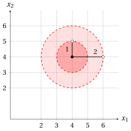
Consider the point \(\bar{\boldsymbol x} = \begin{pmatrix} 4 \\ 4 \end{pmatrix} \in \R^2\) and the radii \(\delta_1=1\) and \(\delta_2=2\). The associated spherical \(\delta\)-neighborhoods
and
are the red disks in the figure: the darker disk is \(N\big(\bar{\boldsymbol x},1\big)\), which is contained in \(N\big(\bar{\boldsymbol x},2\big)\). The boundary circles are dashed because they do not belong to the neighborhoods: for instance, the points \(\begin{pmatrix} 4 \\ 5 \end{pmatrix}\) and \(\begin{pmatrix} 6 \\ 4 \end{pmatrix}\) (empty circles) have distance exactly \(1\) and \(2\) from the center, respectively.
Definition 5.5: point of local minimum/maximum and local minimum/maximum
Given a function \(f:D\subseteq \R^n \rightarrow \R\), a point \(\bar{\boldsymbol x} \in D\) is
-
a point of local minimum of \(f\) in \(D\) if there exists a spherical neighborhood \(N(\bar{\boldsymbol x},\delta)\) with \(\delta \in \R_{>0}\) such that:
\[ f(\bar{\boldsymbol x}) ~\le~ f({\boldsymbol x}),~~~~ \forall {\boldsymbol x} \in N(\bar{\boldsymbol x},\delta) \cap D \]and \(f(\bar{\boldsymbol x})\) is a local minimum of \(f\) in \(D\);
-
a point of local maximum of \(f\) in \(D\) if there exists a spherical neighborhood \(N(\bar{\boldsymbol x},\delta)\) with \(\delta \in \R_{>0}\) such that:
\[ f(\bar{\boldsymbol x}) ~\ge~ f({\boldsymbol x}),~~~~ \forall {\boldsymbol x} \in N(\bar{\boldsymbol x},\delta) \cap D \]and \(f(\bar{\boldsymbol x})\) is a local maximum of \(f\) in \(D\).
-
There can exist multiple points of local minimum (maximum), possibly infinitely many.
-
To prove that a point is a point of local minimum (maximum) with the definition, it is enough to exhibit one radius \(\delta\) for which the inequality holds in \(N(\bar{\boldsymbol x},\delta) \cap D\); any smaller radius also works.
Example 5.13: points of local minimum
Consider the following function:
This is the graph of the function in \([-3,3]\times[-3,3]\); the violet point is \(\big(0,0,f(0,0)\big) = (0,0,0)\).
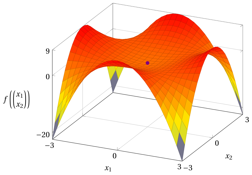
To prove that the point \(\begin{pmatrix}0\\0\end{pmatrix}\) is a point of local minimum, we use the spherical \(\delta\)-neighborhood \(N\!\left(\begin{pmatrix}0\\0\end{pmatrix},1\right)\). For every \(\begin{pmatrix}x_1\\x_2\end{pmatrix}\in N\!\left(\begin{pmatrix}0\\0\end{pmatrix},1\right)\) we have \(x_2^2 \le x_1^2+x_2^2<1\), hence \(1-\dfrac{x_2^2}{2} > \dfrac{1}{2}\), and then:
with equality only for \(x_1=x_2=0\). It follows that
and \(\begin{pmatrix}0\\0\end{pmatrix}\) is a point of local minimum of \(f\) in \(\R^2\), with local minimum \(0\). It is not a point of (global) minimum, since
- Every point of (global) minimum is a point of local minimum (with any \(\delta\)), and every point of (global) maximum is a point of local maximum. The converse is false: a point of local minimum may not be a point of minimum, as the previous example and the following one show.
Example 5.14: a local minimum that is not a global minimum
Consider the following function:
Since \((x+2)^2 \le (x-2)^2+1\) if and only if \(8x \le 1\), we have
In the figure, the points of global minimum and maximum are blue and the other points of local minimum and maximum are violet.
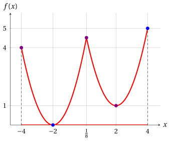
-
Global minimum. Both \((x+2)^2\) and \((x-2)^2+1\) are nonnegative, so \(f(x) \ge 0 = f(-2)\) for every \(x \in [-4,4]\); since \((x-2)^2+1 \ge 1\), \(f(x) = 0\) only for \(x=-2\). The point \(x=-2\) is the unique point of minimum and the minimum is \(0\).
-
Local minimum that is not global. In the neighborhood \(N\big((2),1\big) = (1,3)\) we have \(x \ge \frac{1}{8}\), and then
\[ f(x) = (x-2)^2+1 \ge 1 = f(2), \qquad \forall x \in N\big((2),1\big) \cap [-4,4] = (1,3). \]The point \(x=2\) is a point of local minimum and \(1\) is a local minimum; it is not a point of (global) minimum, since \(f(-2) = 0 < 1 = f(2)\).
-
Global maximum. For \(-4 \le x \le \frac{1}{8}\) we have \(-2 \le x+2 \le \frac{17}{8}\) and then \(f(x) = (x+2)^2 \le \big(\frac{17}{8}\big)^2 = \frac{289}{64} < 5\). For \(\frac{1}{8} \le x \le 4\) we have \(-\frac{15}{8} \le x-2 \le 2\) and then \(f(x) = (x-2)^2+1 \le 4+1 = 5\), with equality only for \(x=4\). The point \(x=4\) is the unique point of maximum and the maximum is \(5\).
-
Local maxima that are not global. In \(N\big((-4),1\big) \cap [-4,4] = [-4,-3)\) we have \(-2 \le x+2 < -1\) and then \(f(x) = (x+2)^2 \le 4 = f(-4)\): the point \(x=-4\) is a point of local maximum. In \(N\big((\frac{1}{8}),1\big) = (-\frac{7}{8},\frac{9}{8})\) we have \(0 < x+2 \le \frac{17}{8}\) when \(x \le \frac{1}{8}\), so that \(f(x) = (x+2)^2 \le \frac{289}{64}\), and \(-\frac{15}{8} \le x-2 < 0\) when \(x \ge \frac{1}{8}\), so that \(f(x) = (x-2)^2+1 \le \frac{225}{64}+1 = \frac{289}{64}\); in both cases \(f(x) \le f(\frac{1}{8})\): the point \(x=\frac{1}{8}\) is a point of local maximum. Neither of them is a point of (global) maximum, since \(f(-4) = 4 < 5\) and \(f(\frac{1}{8}) = \frac{289}{64} < 5\).
Consider the optimization problem \(\min \{\, f(x) \text{ subject to } -4 \le x \le 4 \,\}\): a method that only looks at the points close to \(x=2\) finds the local minimum \(1\), but the optimal value is \(z(P) = 0\), attained at \(\tilde{\boldsymbol x}(P) = (-2)\).
Exercises on this chapter: Optimization problems
Interactive lab
The ideas of the chapter, hands on: move the sliders and drag the points. All the graphs of the course are in the interactive lab.