Functions of several variables¶

Part 1 · Preliminaries · Chapter 2 · Lecture notes, volume 1 (PDF) · Slides · Exercises: Functions of several variables · App: Level sets and gradient

2.1 Functions of several variables¶

Definition 2.1: function of several real variables

The function:

\[\begin{equation*} f: D \subseteq \R^n \rightarrow \mathbb{R},~~~ f: \underbrace{ \begin{pmatrix} x_1 \\ x_2 \\ \vdots \\ x_n \end{pmatrix} }_{{\boldsymbol x}} \mapsto f({\boldsymbol x}) \end{equation*}\]

is called a (scalar) function of \(n\) real variables and \(D \subseteq \R^n\) is its domain.

A function, commonly denoted \(f\), of \(n\) real variables takes as input a vector of \(n\) real numbers, commonly represented by the (column) variable vector \({\boldsymbol x}\), and produces a real number, the value of the function, commonly denoted \(f({\boldsymbol x})\).
Vectors are written in bold and are column vectors; the transpose of a vector \({\boldsymbol x}\) is the row vector \({\boldsymbol x}' = \begin{pmatrix} x_1 & x_2 & \dots & x_n \end{pmatrix}\).

Example 2.1: a function of three variables

Consider the function:

\[ f: \R^3 \rightarrow \R,~~ f: \begin{pmatrix} x_1 \\ x_2 \\ x_3 \end{pmatrix} \mapsto x_1\,x_2 + x_3^2 \]

At the point \(\begin{pmatrix} 2 \\ -1 \\ 3 \end{pmatrix}\) the value of the function is:

\[ f\left(\begin{pmatrix} 2 \\ -1 \\ 3 \end{pmatrix}\right) = 2 \cdot (-1) + 3^2 = -2 + 9 = 7 \]

2.2 Gradient, Hessian and level sets¶

Definition 2.2: gradient

Given \(f:D\subseteq \R^n \to \R\), the gradient \(\nabla f(\boldsymbol x)\) of \(f\) at \(\boldsymbol x\) is the (column) vector of first-order partial derivatives:

\[ \nabla f(\boldsymbol x) := \begin{pmatrix} \frac{\partial f(\boldsymbol x)}{\partial x_1}\\[1ex] \frac{\partial f(\boldsymbol x)}{\partial x_2}\\[1ex] \vdots\\[1ex] \frac{\partial f(\boldsymbol x)}{\partial x_n} \end{pmatrix} \]

The gradient \(\nabla f(\boldsymbol x)\) (if it is nonzero) gives the direction of steepest ascent (maximum directional derivative among unit directions), while \(-\nabla f(\boldsymbol x)\) gives the direction of steepest descent.

Definition 2.3: Hessian

Given a function \(f:D\subseteq \R^n \to \R\), the Hessian \(\nabla^2 f(\boldsymbol x)\) of \(f\) at \(\boldsymbol x\) is the matrix of second-order partial derivatives:

\[ \nabla^2 f(\boldsymbol x) := \begin{pmatrix} \frac{\partial^2 f(\boldsymbol x)}{\partial x_1^2} & \frac{\partial^2 f(\boldsymbol x)}{\partial x_1\partial x_2} & \dots & \frac{\partial^2 f(\boldsymbol x)}{\partial x_1\partial x_n}\\[2ex] \frac{\partial^2 f(\boldsymbol x)}{\partial x_2\partial x_1} & \frac{\partial^2 f(\boldsymbol x)}{\partial x_2^2} & \dots & \frac{\partial^2 f(\boldsymbol x)}{\partial x_2\partial x_n}\\[2ex] \vdots & \vdots & \ddots & \vdots\\[2ex] \frac{\partial^2 f(\boldsymbol x)}{\partial x_n\partial x_1} & \frac{\partial^2 f(\boldsymbol x)}{\partial x_n\partial x_2} & \dots & \frac{\partial^2 f(\boldsymbol x)}{\partial x_n^2} \end{pmatrix} \]

The entry in row \(i\) and column \(j\) of the Hessian is obtained by differentiating \(\frac{\partial f(\boldsymbol x)}{\partial x_j}\) with respect to \(x_i\).
If the second-order partial derivatives of \(f\) are continuous (as for all the functions of these notes), the order of differentiation does not matter, \(\frac{\partial^2 f(\boldsymbol x)}{\partial x_i\partial x_j} = \frac{\partial^2 f(\boldsymbol x)}{\partial x_j\partial x_i}\), and the Hessian is a symmetric matrix.

The Hessian \(\nabla^2 f(\boldsymbol x)\) describes the local curvature of \(f\) around \(\boldsymbol x\), that is, how the gradient changes when moving away from \(\boldsymbol x\).

Definition 2.4: level set

Given a function \(f:D\subseteq \R^n \to \R\) and a constant \(k\in\R\), the level set \(L(k)\) of \(f\) at level \(k\) is:

\[ L(k) := \{\, \boldsymbol x \in D : f(\boldsymbol x)=k \,\} \]

A level set \(L(k)\) is the set of points where the function has a constant value \(k\). The gradient \(\nabla f(\boldsymbol x)\) (if nonzero) is perpendicular to the level set passing through \(\boldsymbol x\) and points toward increasing values of \(f\).

Example 2.2: gradient, Hessian and level sets of a quadratic function

Consider the quadratic function:

\[ f: \R^2 \rightarrow \R,~~f: \begin{pmatrix} x_1 \\ x_2 \end{pmatrix} \mapsto (x_1-2)^2 + (x_2-2)^2 +1 \]

The gradient of the function is:

\[ \nabla f\left(\begin{pmatrix} x_1 \\ x_2 \end{pmatrix}\right) = \begin{pmatrix} \frac{ \partial f}{ \partial x_1} \\[2ex] \frac{ \partial f}{ \partial x_2} \end{pmatrix} = \begin{pmatrix} 2(x_1-2) \\[1ex] 2(x_2-2) \end{pmatrix} \]

For example:
- at the point \(\begin{pmatrix} 3 \\ 2 \end{pmatrix}\), we have
  
  \[ \nabla f\left(\begin{pmatrix} 3 \\ 2 \end{pmatrix}\right) = \begin{pmatrix} 2(3-2) \\ 2(2-2) \end{pmatrix} = \begin{pmatrix} 2 \\ 0 \end{pmatrix} \]
- at the point \(\begin{pmatrix} 2 \\ 3 \end{pmatrix}\), we have
  
  \[ \nabla f\left(\begin{pmatrix} 2 \\ 3 \end{pmatrix}\right) = \begin{pmatrix} 2(2-2) \\ 2(3-2) \end{pmatrix} = \begin{pmatrix} 0 \\ 2 \end{pmatrix} \]
The Hessian of the function is:

\[ \nabla^2 f\left(\begin{pmatrix} x_1 \\ x_2 \end{pmatrix}\right) = \begin{pmatrix} \frac{ \partial^2 f}{ \partial x_1^2} & \frac{ \partial^2 f}{ \partial x_1 \partial x_2} \\[2ex] \frac{ \partial^2 f}{ \partial x_2 \partial x_1} & \frac{ \partial^2 f}{ \partial x_2^2} \end{pmatrix} = \begin{pmatrix} 2 & 0 \\[1ex] 0 & 2 \end{pmatrix} \]

Note that the Hessian is constant (it does not depend on the point).
The level sets of the function are:

\[ L(k) = \left\{~\begin{pmatrix} x_1 \\ x_2 \end{pmatrix} \in \R^2:~ (x_1-2)^2 + (x_2-2)^2 +1= k ~\right\} , \qquad \forall k \in \mathbb{R} \]

which are circles centered at \(\begin{pmatrix} 2 \\ 2 \end{pmatrix}\) with radius \(\sqrt{k-1}\) for \(k > 1\); the level set \(L(1)\) is the single point \(\begin{pmatrix} 2 \\ 2 \end{pmatrix}\) and the level sets with \(k<1\) are empty.

Example 2.3: graph, level sets and gradients of a quadratic function

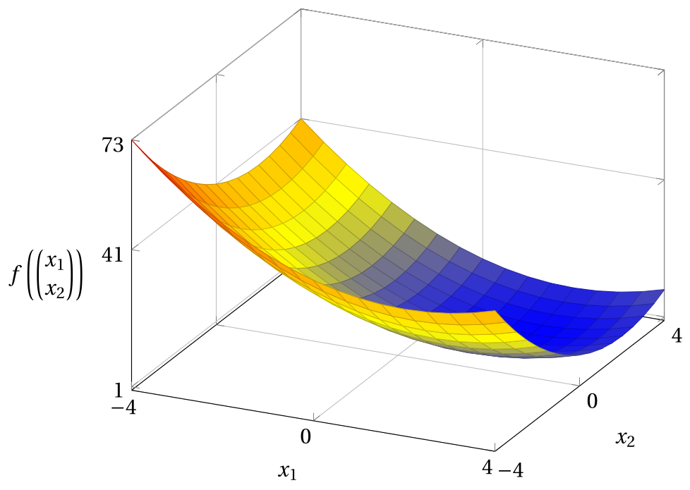
For the function of the previous example, this is the graph in the domain \([-4,4]\times[-4,4]\); its lowest point is at \(\begin{pmatrix} 2 \\ 2 \end{pmatrix}\), where \(f = 1\), and its highest point is at \(\begin{pmatrix} -4 \\ -4 \end{pmatrix}\), where \(f = 73\):

The following figure shows the level sets \(L(2)\) (circle of radius \(1\), in blue) and \(L(17)\) (circle of radius \(4\), in orange), and the two gradients of the previous example (in red), drawn from the points \(\begin{pmatrix} 3 \\ 2 \end{pmatrix}\) and \(\begin{pmatrix} 2 \\ 3 \end{pmatrix}\) of the level set \(L(2)\):

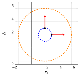
The gradient vectors are perpendicular to the level sets and point in the direction of maximum increase of the function (away from the center).

2.3 Examples of functions that are not quadratic¶

For a quadratic function the Hessian is constant (chapter «Quadratic functions»). In general, the Hessian depends on the point, as in the following two examples.

Example 2.4: gradient and Hessian of a cubic function

Consider the function:

\[ f: \R^2 \rightarrow \R,~~f: \begin{pmatrix} x_1 \\ x_2 \end{pmatrix} \mapsto x_1^2\,x_2 \]

The gradient and the Hessian of the function are:

\[ \nabla f\left(\begin{pmatrix} x_1 \\ x_2 \end{pmatrix}\right) = \begin{pmatrix} 2\,x_1 x_2 \\[1ex] x_1^2 \end{pmatrix}, \qquad \nabla^2 f\left(\begin{pmatrix} x_1 \\ x_2 \end{pmatrix}\right) = \begin{pmatrix} 2\,x_2 & 2\,x_1 \\[1ex] 2\,x_1 & 0 \end{pmatrix} \]
At the point \(\begin{pmatrix} 1 \\ 2 \end{pmatrix}\), we have:

\[ \nabla f\left(\begin{pmatrix} 1 \\ 2 \end{pmatrix}\right) = \begin{pmatrix} 2 \cdot 1 \cdot 2 \\[0.5ex] 1^2 \end{pmatrix} = \begin{pmatrix} 4 \\ 1 \end{pmatrix}, \qquad \nabla^2 f\left(\begin{pmatrix} 1 \\ 2 \end{pmatrix}\right) = \begin{pmatrix} 4 & 2 \\ 2 & 0 \end{pmatrix} \]
At the point \(\begin{pmatrix} -1 \\ 3 \end{pmatrix}\), we have:

\[ \nabla f\left(\begin{pmatrix} -1 \\ 3 \end{pmatrix}\right) = \begin{pmatrix} 2 \cdot (-1) \cdot 3 \\[0.5ex] (-1)^2 \end{pmatrix} = \begin{pmatrix} -6 \\ 1 \end{pmatrix}, \qquad \nabla^2 f\left(\begin{pmatrix} -1 \\ 3 \end{pmatrix}\right) = \begin{pmatrix} 6 & -2 \\ -2 & 0 \end{pmatrix} \]

The Hessian changes from point to point and, as expected, it is symmetric at every point.

Example 2.5: gradient, Hessian and a level set of an exponential function

Consider the function:

\[ f: \R^2 \rightarrow \R,~~f: \begin{pmatrix} x_1 \\ x_2 \end{pmatrix} \mapsto e^{x_1} + x_2^2 \]

The gradient and the Hessian of the function are:

\[ \nabla f\left(\begin{pmatrix} x_1 \\ x_2 \end{pmatrix}\right) = \begin{pmatrix} e^{x_1} \\[1ex] 2\,x_2 \end{pmatrix}, \qquad \nabla^2 f\left(\begin{pmatrix} x_1 \\ x_2 \end{pmatrix}\right) = \begin{pmatrix} e^{x_1} & 0 \\[1ex] 0 & 2 \end{pmatrix} \]
The level set \(L(2)\) is the curve \(e^{x_1} + x_2^2 = 2\), that is, \(x_1 = \ln(2 - x_2^2)\) for \(|x_2| < \sqrt{2}\). It contains the points \(\begin{pmatrix} 0 \\ 1 \end{pmatrix}\) and \(\begin{pmatrix} \ln 2 \\ 0 \end{pmatrix}\), since \(e^0 + 1^2 = 2\) and \(e^{\ln 2} + 0^2 = 2\). At these points:

\[ \nabla f\left(\begin{pmatrix} 0 \\ 1 \end{pmatrix}\right) = \begin{pmatrix} 1 \\ 2 \end{pmatrix}, \qquad \nabla f\left(\begin{pmatrix} \ln 2 \\ 0 \end{pmatrix}\right) = \begin{pmatrix} 2 \\ 0 \end{pmatrix} \]

and

\[ \nabla^2 f\left(\begin{pmatrix} 0 \\ 1 \end{pmatrix}\right) = \begin{pmatrix} 1 & 0 \\ 0 & 2 \end{pmatrix}, \qquad \nabla^2 f\left(\begin{pmatrix} \ln 2 \\ 0 \end{pmatrix}\right) = \begin{pmatrix} 2 & 0 \\ 0 & 2 \end{pmatrix} \]

The following figure shows the level set \(L(2)\) (in blue) and the two gradient vectors (in red):

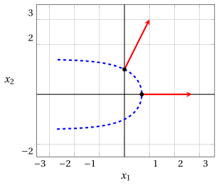
The tangent direction of the level set at \(\begin{pmatrix} 0 \\ 1 \end{pmatrix}\) is \(\begin{pmatrix} -2 \\ 1 \end{pmatrix}\) (the derivative of \(x_1 = \ln(2-x_2^2)\) with respect to \(x_2\) is \(\frac{-2\,x_2}{2-x_2^2}\), equal to \(-2\) at \(x_2=1\)), and indeed:

\[ \begin{pmatrix} 1 & 2 \end{pmatrix} \begin{pmatrix} -2 \\ 1 \end{pmatrix} = -2 + 2 = 0 \]

so the gradient is perpendicular to the level set also when the level set is not a circle.

The gradient \(\nabla f(\boldsymbol x)\) is the column vector of first-order partial derivatives: it points in the direction of steepest ascent and is perpendicular to the level set through \(\boldsymbol x\). The Hessian \(\nabla^2 f(\boldsymbol x)\) is the (symmetric) matrix of second-order partial derivatives and describes the local curvature of \(f\).

Exercises on this chapter: Functions of several variables

Interactive lab¶

The ideas of the chapter, hands on: move the sliders and drag the points. All the graphs of the course are in the interactive lab.