Support Vector Machine: optimization for machine learning
Lecture notes (PDF) · Chapter slides (PDF)
Class: convex QP · Script: python/lab15_svm.py

The SVM connects convex optimization to machine learning: the classifier is obtained by solving a QP. Here no ML libraries: every model is a QP written and solved with Gurobi, in order to understand what a classifier optimizes. The labels \(y_i \in \{-1, +1\}\) are data; the variables (coefficients, intercept, slacks, multipliers) are all continuous.
Hard margin
Data (input of the model).
| Symbol | Type | Meaning |
|---|---|---|
| \(n\) | \(\in \mathbb{Z}_{\ge 1}\) | number of observations of the training set, indexed by \(i \in \{1, 2, \dots, n\}\) |
| \(p\) | \(\in \mathbb{Z}_{\ge 1}\) | number of features, indexed by \(j \in \{1, 2, \dots, p\}\) |
| \(x_{ij}\) | \(\in \mathbb{Q}\) | value of feature \(j\) for observation \(i\); \(\boldsymbol x_i \in \mathbb{Q}^p\) is the vector of observation \(i\) |
| \(y_i\) | \(\in \{-1, +1\}\) | observed class label of \(i\) (a datum, not a variable) |
| \(C\) | \(\in \mathbb{Q}_{> 0}\) | weight of the margin violations (soft margin only); upper case to follow the machine learning literature, an exception to the convention that reserves capital letters for sets and matrices |
Decision variables. We introduce the following \(p + 1\) free variables:
which define the hyperplane \(\sum_{j=1}^{p} w_j\, x_j + b = 0\). Using these variables, the hard margin QP model is the following:
Description of the objective function and of the constraints:
- the convex quadratic objective function minimizes \(\tfrac12\|\boldsymbol w\|^2\); since the geometric margin between the supporting hyperplanes is \(2/\|\boldsymbol w\|\), minimizing it is equivalent to maximizing the margin;
- the linear classification constraints impose that every observation lies on the right side of the hyperplane, at a distance of at least one unit in the scale of \(\boldsymbol w\) (\(n\) linear constraints);
- the constraints on \(w_j\) and \(b\) define the variables of the model, all free.
Worked example by hand (2 points)
\(\boldsymbol x_1 = (0.0)\), \(y_1 = -1\); \(\boldsymbol x_2 = (2.2)\), \(y_2 = +1\): \(\boldsymbol w = (0{,}5;\, 0{,}5)\), \(b = -1\), margin \(2/\|\boldsymbol w\| = 2\sqrt2 = 2{,}83\) = the distance between the points; both constraints are active, hence both points are support vectors.
Soft margin and the role of C
With real overlapping data the hard margin is infeasible: one adds \(n\) non-negative slack variables,
where \(\xi_i > 1\) corresponds to a misclassification.
Description of the objective function and of the constraints:
- the convex quadratic objective function balances two terms: the simplicity of the model (\(\tfrac12\|\boldsymbol w\|^2\), wide margin) and the cost of the violations on the training set (\(C \sum_{i=1}^{n} \xi_i\)); \(C\) is the price assigned to the violations;
- the linear classification constraints require correct classification up to the slack \(\xi_i\), paid in the objective (\(n\) linear constraints);
- the constraints on \(w_j\), \(b\) and \(\xi_i\) define the variables of the model: \(w_j\) and \(b\) free, \(\xi_i\) non-negative.
Case study: 90 customers described by two standardized indicators (capital soundness,
punctuality of payments), 55 creditworthy and 35 defaulting, partially overlapping
(data/svm_clienti.csv).
C =  0.05: w = (0.678, 0.474)  b = -0.148 | margin 2.418 | errors 2 | in the margin 22
C =  1.00: w = (1.433, 0.611)  b = -0.236 | margin 1.284 | errors 2 | in the margin  7
C = 20.00: w = (5.058, 2.338)  b = -2.936 | margin 0.359 | errors 0 | in the margin  3
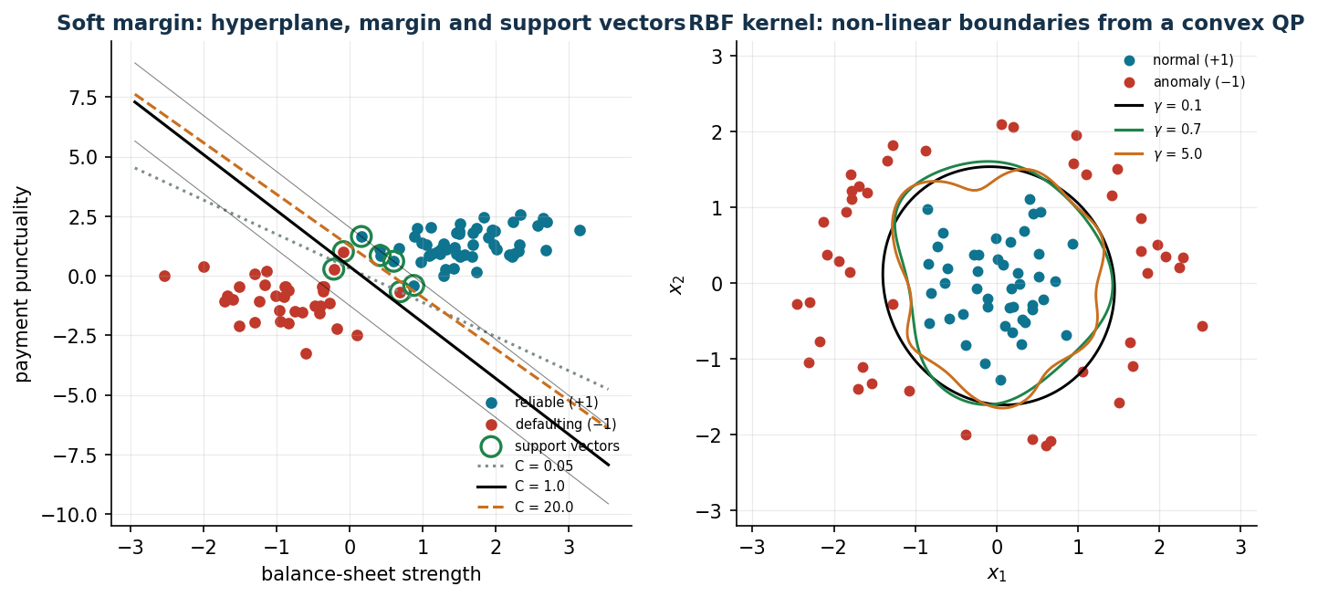
A small \(C\) buys a wide margin while accepting 22 points inside the margin; a large \(C\) chases every point of the training set (zero errors, a very narrow margin): this is the regularization–fit trade-off, and it must be chosen with validation data, never by looking at the test set.
The dual and the support vectors
By associating a multiplier \(\alpha_i\) with each classification constraint of the soft margin, one obtains \(n\) new variables:
Description of the objective function and of the constraints:
- the concave quadratic objective function depends on the data only through the inner products \(\boldsymbol x_i' \boldsymbol x_j\): this is the observation that opens the door to the kernel;
- the linear stationarity constraint follows from the derivative with respect to the intercept \(b\) (one linear constraint);
- the constraints \(\alpha_i \le C\) bound each multiplier by the price \(C\) of the violations (\(n\) linear constraints);
- the non-negativity constraints on \(\alpha_i\) define the variables of the model.
Primal-dual relation: \(\boldsymbol w = \sum_{i=1}^{n} \alpha_i\, y_i\, \boldsymbol x_i\) and \(f(\boldsymbol x) = \mathrm{sign}(\boldsymbol w' \boldsymbol x + b)\).
w from the dual = (1.433, 0.611)   b = -0.236     (identical to the primal)
dual value 4.7868 = primal value (strong duality)
alpha = 0        : 83 points  -> do NOT affect the boundary
0 < alpha < C    :  2 points  -> support vectors exactly on the margin
alpha = C        :  5 points  -> inside the margin or misclassified
The solution depends only on the 7 points with \(\alpha_i > 0\): it is they that "support" the hyperplane, the other 83 could disappear without changing anything. The KKT complementarity organizes everything: \(\alpha_i = 0 \Rightarrow\) point beyond the margin; \(0 < \alpha_i < C \Rightarrow\) exactly on the margin (from these one recovers \(b\)); \(\alpha_i = C \Rightarrow\) the constraint "pays" a slack \(\xi_i > 0\). And the dual depends on the data only through the inner products: the door to the kernel.
RBF kernel
By replacing \(\boldsymbol x_i'\boldsymbol x_j\) with a kernel \(K(\boldsymbol x_i, \boldsymbol x_j)\) — for example the Gaussian RBF (Radial Basis Function) kernel \(K(\boldsymbol x, \boldsymbol z) = e^{-\gamma\|\boldsymbol x - \boldsymbol z\|^2}\) — one classifies in a transformed space without ever building it: \(f(\boldsymbol x) = \mathrm{sign}\bigl(\sum_{i=1}^{n} \alpha_i y_i K(\boldsymbol x_i, \boldsymbol x) + b\bigr)\). The boundary can be arbitrarily curved, but the training problem remains a convex QP if the kernel is valid (positive semidefinite matrix). Case study: 90 process observations, normal operation in the centre and anomalies arranged in a ring — no straight line can separate them.
gamma = 0.1: training errors  1   support vectors 20
gamma = 0.7: training errors  0   support vectors 15
gamma = 5.0: training errors  0   support vectors 61  <- "memorizes" the points
With \(\gamma = 5\) the boundary breaks up into islands around the individual points and the support vectors rise to 61 out of 90: the model is memorizing the training set (overfitting), while still remaining a convex QP. Convexity of training and the ability to generalize are different properties: \(C\) and \(\gamma\) must be chosen together by cross-validation.
Unbalanced classes and SVR
In managerial applications the important class is rare and an error on the rare cases costs more. It is enough to weight the slacks: \(C_-\sum_{i:\, y_i = -1}\xi_i + C_+\sum_{i:\, y_i = +1}\xi_i\).
equal costs (C=1)           : precision 1.00   recall defaulters 0.94
10x cost on the defaulters  : precision 0.97   recall defaulters 1.00
With the 10× cost the boundary moves back towards the "healthy" class: no defaulter escapes (recall 100%) at the price of a few more false alarms (precision from 100% to 97%). The weights must reflect the decision costs, not the frequencies of the classes.
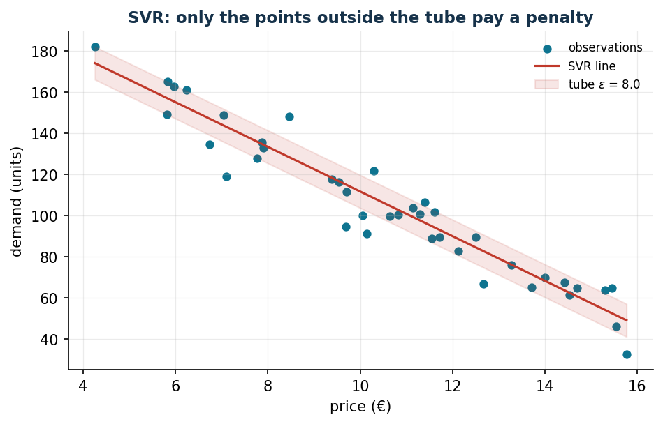
SVR: Support Vector Regression estimates a continuous function while ignoring the errors within a tube of width \(\varepsilon\), that is, \(\min \tfrac12\|\boldsymbol w\|^2 + C\sum_{i=1}^{n} (\xi_i + \xi_i^*)\) with \(|y_i - (\boldsymbol w' \boldsymbol x_i + b)| \le \varepsilon + \xi_i^{(*)}\) for every \(i \in \{1, 2, \dots, n\}\).
SVR line: demand = -10.86 * price + 220.32    (true: -11p + 220)
Tube eps = 8: 14 points out of 40 outside the tube -> only they determine the line
Code
The complete script of the chapter — data, model, solution, sensitivity and figures —
is python/lab15_svm.py
(reproducible with python3 python/lab15_svm.py from the python/ folder).
The same code is also available as a notebook — notebooks/lab15_svm.ipynb — which opens in Colab from the badge at the top of the page and runs in the browser, with nothing to install.
Show the full script — lab15_svm.py
"""Chapter 15 — Support Vector Machine as a convex QP (no sklearn: everything in Gurobi).

Case study: credit risk. 90 customers described by two standardised indicators:
x1 = balance-sheet strength, x2 = punctuality in payments.
Label y = +1 reliable customer, y = -1 defaulting customer.

Contents:
  1. Hard margin on separable data (QP)
  2. Soft margin as C varies; support vectors and violations
  3. Dual formulation: alpha, reconstruction of w and b, complementarity
  4. RBF kernel: non-linear boundary (dual QP)
  5. Imbalanced classes: asymmetric costs C+ / C-
  6. Support Vector Regression on price -> demand
"""
import gurobipy as gp
import numpy as np
import pandas as pd
from gurobipy import GRB

from stile import (ARANCIO, GRIGIO, ROSSO, TEAL, VERDE, intestazione, plt, salva_dat,
                   salva_dati, salva_figura, salva_tikz)

rng = np.random.default_rng(11)

# ----------------------------------------------------------------------
# 1. DATA: two partially overlapping groups of customers
# ----------------------------------------------------------------------
n_pos, n_neg = 55, 35
X_pos = rng.multivariate_normal([1.6, 1.4], [[0.55, 0.15], [0.15, 0.45]], n_pos)
X_neg = rng.multivariate_normal([-0.9, -1.1], [[0.65, -0.1], [-0.1, 0.7]], n_neg)
X = np.vstack([X_pos, X_neg])
y = np.array([1.0] * n_pos + [-1.0] * n_neg)
n = len(y)
salva_dati(pd.DataFrame({"x1": X[:, 0], "x2": X[:, 1], "y": y}), "svm_clienti")


def svm_primale(C, pesi=None):
    """Primal soft margin: min 1/2||w||^2 + sum C_i xi_i."""
    Ci = np.full(n, C) if pesi is None else pesi
    m = gp.Model("svm_primal")
    m.Params.OutputFlag = 0
    w = m.addVars(2, lb=-GRB.INFINITY, name="w")
    b = m.addVar(lb=-GRB.INFINITY, name="b")
    xi = m.addVars(n, name="xi")
    m.addConstrs((y[i] * (w[0] * X[i, 0] + w[1] * X[i, 1] + b) >= 1 - xi[i]
                  for i in range(n)), name="classif")
    m.setObjective(0.5 * (w[0] * w[0] + w[1] * w[1])
                   + gp.quicksum(Ci[i] * xi[i] for i in range(n)), GRB.MINIMIZE)
    m.optimize()
    assert m.Status == GRB.OPTIMAL
    return (np.array([w[0].X, w[1].X]), b.X,
            np.array([xi[i].X for i in range(n)]), m.ObjVal)


# ----------------------------------------------------------------------
# 2. SOFT MARGIN AS C VARIES
# ----------------------------------------------------------------------
intestazione("Primal soft margin as C varies")
risultati = {}
for C in [0.05, 1.0, 20.0]:
    w, b, xi, obj = svm_primale(C)
    margine = 2 / np.linalg.norm(w)
    err = int(np.sum(y * (X @ w + b) < 0))
    nsv = int(np.sum(y * (X @ w + b) < 1 + 1e-6))
    risultati[C] = (w, b)
    print(f"  C = {C:5.2f}: w = ({w[0]:6.3f}, {w[1]:6.3f}), b = {b:6.3f} | "
          f"margin = {margine:5.3f} | errors = {err:2d} | points inside the margin = {nsv:2d}")
print("Small C -> wide margin and more violations; large C -> narrow margin.")

C_rif = 1.0
w1, b1, xi1, _ = svm_primale(C_rif)

# ----------------------------------------------------------------------
# 3. DUAL FORMULATION
# ----------------------------------------------------------------------
intestazione(f"Dual with C = {C_rif}")
K_lin = X @ X.T
md = gp.Model("svm_dual")
md.Params.OutputFlag = 0
al = md.addVars(n, ub=C_rif, name="alpha")
md.addConstr(gp.quicksum(al[i] * y[i] for i in range(n)) == 0, name="sum")
md.setObjective(gp.quicksum(al[i] for i in range(n))
                - 0.5 * gp.quicksum(al[i] * al[j] * y[i] * y[j] * K_lin[i, j]
                                    for i in range(n) for j in range(n)), GRB.MAXIMIZE)
md.optimize()
assert md.Status == GRB.OPTIMAL
alpha = np.array([al[i].X for i in range(n)])
w_dual = (alpha * y) @ X
sv_margine = [i for i in range(n) if 1e-5 < alpha[i] < C_rif - 1e-5]
b_dual = float(np.mean([y[i] - w_dual @ X[i] for i in sv_margine]))
print(f"w from the dual = ({w_dual[0]:.3f}, {w_dual[1]:.3f})  (primal: "
      f"({w1[0]:.3f}, {w1[1]:.3f}))")
print(f"b from the dual = {b_dual:.3f}  (primal: {b1:.3f})")
n_zero = int(np.sum(alpha < 1e-5))
n_marg = len(sv_margine)
n_C = int(np.sum(alpha > C_rif - 1e-5))
print(f"alpha = 0 (outside the margin): {n_zero} points — they do NOT affect the boundary")
print(f"0 < alpha < C (on the margin)  : {n_marg} support vectors")
print(f"alpha = C (inside/beyond)      : {n_C} points with xi > 0")
print(f"Dual value = {md.ObjVal:.4f} (equal to the primal one by strong duality)")

sv = alpha > 1e-5
salva_dat(pd.DataFrame({"x1": X[:, 0], "x2": X[:, 1], "y": y,
                        "alpha": alpha, "sv": sv.astype(int)}), "cap14_punti")
salva_dat(pd.DataFrame({"C": [0.05, 1.0, 20.0],
                        "w1": [risultati[C][0][0] for C in [0.05, 1.0, 20.0]],
                        "w2": [risultati[C][0][1] for C in [0.05, 1.0, 20.0]],
                        "b": [risultati[C][1] for C in [0.05, 1.0, 20.0]]}), "cap14_rette")

# ----------------------------------------------------------------------
# 4. RBF KERNEL
# ----------------------------------------------------------------------
intestazione("RBF kernel (ring-shaped data: not linearly separable)")
# second dataset: process anomalies around a normal operating region
n2a, n2b = 45, 45
raggi = rng.normal(0, 0.55, (n2a, 2))
angoli = rng.uniform(0, 2 * np.pi, n2b)
corona = np.column_stack([(2.0 + rng.normal(0, 0.25, n2b)) * np.cos(angoli),
                          (2.0 + rng.normal(0, 0.25, n2b)) * np.sin(angoli)])
X2 = np.vstack([raggi, corona])
y2 = np.array([1.0] * n2a + [-1.0] * n2b)
n2 = len(y2)
salva_dati(pd.DataFrame({"x1": X2[:, 0], "x2": X2[:, 1], "y": y2}), "svm_corona")
salva_dat(pd.DataFrame({"x1": X2[:, 0], "x2": X2[:, 1], "y": y2}), "cap14_corona")


def svm_rbf(gamma, C=5.0):
    K = np.exp(-gamma * ((X2[:, None, :] - X2[None, :, :]) ** 2).sum(-1))
    m = gp.Model("rbf")
    m.Params.OutputFlag = 0
    al = m.addVars(n2, ub=C, name="alpha")
    m.addConstr(gp.quicksum(al[i] * y2[i] for i in range(n2)) == 0)
    m.setObjective(gp.quicksum(al[i] for i in range(n2))
                   - 0.5 * gp.quicksum(al[i] * al[j] * y2[i] * y2[j] * K[i, j]
                                       for i in range(n2) for j in range(n2)), GRB.MAXIMIZE)
    m.optimize()
    aa = np.array([al[i].X for i in range(n2)])
    svm_ = [i for i in range(n2) if 1e-5 < aa[i] < C - 1e-5]
    bb = float(np.mean([y2[i] - sum(aa[j] * y2[j] * K[j, i] for j in range(n2))
                        for i in svm_]))

    def punteggio(P):
        KK = np.exp(-gamma * ((P[:, None, :] - X2[None, :, :]) ** 2).sum(-1))
        return KK @ (aa * y2) + bb

    err = int(np.sum(punteggio(X2) * y2 < 0))
    return punteggio, aa, err


griglia = np.linspace(-3.2, 3.2, 120)
GX, GY = np.meshgrid(griglia, griglia)
P_griglia = np.column_stack([GX.ravel(), GY.ravel()])
contorni = {}
for gamma in [0.1, 0.7, 5.0]:
    punteggio, aa, err = svm_rbf(gamma)
    Z = punteggio(P_griglia).reshape(GX.shape)
    contorni[gamma] = Z
    print(f"  gamma = {gamma:4.1f}: training errors = {err:2d}, "
          f"support vectors = {int(np.sum(aa > 1e-5)):2d}")
print("Small gamma -> smooth boundary; large gamma -> a boundary that 'memorises'.")

# export the boundary (level 0) for pgfplots
for gamma in [0.1, 0.7, 5.0]:
    cs = plt.contour(GX, GY, contorni[gamma], levels=[0.0])
    segmenti = []
    for percorso in cs.allsegs[0]:
        for px, py in percorso:
            segmenti.append((px, py))
        segmenti.append((np.nan, np.nan))       # line separator for pgfplots
    plt.close()
    salva_dat(pd.DataFrame(segmenti, columns=["x", "y"]),
              f"cap14_rbf_g{str(gamma).replace('.', '_')}")

# ----------------------------------------------------------------------
# 5. IMBALANCED CLASSES: asymmetric costs
# ----------------------------------------------------------------------
intestazione("Imbalanced classes: missing a defaulter costs 10 times as much")


def metriche(w, b, XX, yy):
    pred = np.sign(XX @ w + b)
    tp = np.sum((pred == -1) & (yy == -1))     # defaulters detected
    fp = np.sum((pred == -1) & (yy == 1))
    fn = np.sum((pred == 1) & (yy == -1))
    prec = tp / (tp + fp) if tp + fp else 0
    rec = tp / (tp + fn) if tp + fn else 0
    return prec, rec


pesi_eq = np.full(n, 1.0)
pesi_asim = np.where(y == -1, 10.0, 1.0)
for nome, pesi in [("equal costs (C = 1)", pesi_eq), ("10x cost on defaulters", pesi_asim)]:
    w, b, xi, _ = svm_primale(1.0, pesi=pesi)
    prec, rec = metriche(w, b, X, y)
    print(f"  {nome:>26}: precision = {prec:.2f}, recall on defaulters = {rec:.2f}")
print("Weighting the rare class more shifts the boundary: more false alarms are accepted")
print("in order not to let a defaulter through.")

# ----------------------------------------------------------------------
# 6. SUPPORT VECTOR REGRESSION: demand as a function of price
# ----------------------------------------------------------------------
intestazione("SVR: estimating the price -> demand curve")
np_srv = 40
prezzi = rng.uniform(4, 16, np_srv)
domanda_v = 220 - 11 * prezzi + rng.normal(0, 9, np_srv)
salva_dati(pd.DataFrame({"price": prezzi, "demand": domanda_v}), "svr_vendite")

eps_svr, C_svr = 8.0, 10.0
ms = gp.Model("svr")
ms.Params.OutputFlag = 0
w_s = ms.addVar(lb=-GRB.INFINITY, name="w")
b_s = ms.addVar(lb=-GRB.INFINITY, name="b")
xi_p = ms.addVars(np_srv, name="xip")
xi_m = ms.addVars(np_srv, name="xim")
ms.addConstrs((domanda_v[i] - (w_s * prezzi[i] + b_s) <= eps_svr + xi_p[i]
               for i in range(np_srv)))
ms.addConstrs(((w_s * prezzi[i] + b_s) - domanda_v[i] <= eps_svr + xi_m[i]
               for i in range(np_srv)))
ms.setObjective(0.5 * w_s * w_s + C_svr * gp.quicksum(xi_p[i] + xi_m[i]
                                                      for i in range(np_srv)), GRB.MINIMIZE)
ms.optimize()
fuori = int(sum(1 for i in range(np_srv)
                if abs(domanda_v[i] - (w_s.X * prezzi[i] + b_s.X)) > eps_svr + 1e-6))
print(f"SVR line: demand = {w_s.X:.2f} · price + {b_s.X:.2f} (true: -11 p + 220)")
print(f"Epsilon tube = {eps_svr}: {fuori} points outside the tube out of {np_srv} "
      f"(only these determine the line)")
salva_dat(pd.DataFrame({"price": prezzi, "demand": domanda_v,
                        "estimate": w_s.X * prezzi + b_s.X}), "cap14_svr")
salva_dat(pd.DataFrame({"w": [w_s.X], "b": [b_s.X], "eps": [eps_svr]}), "cap14_svr_retta")

# ----------------------------------------------------------------------
# 7. FIGURES (matplotlib preview)
# ----------------------------------------------------------------------
fig, (ax1, ax2) = plt.subplots(1, 2, figsize=(10.8, 4.6))
ax1.scatter(X[y > 0, 0], X[y > 0, 1], color=TEAL, s=26, label="reliable (+1)")
ax1.scatter(X[y < 0, 0], X[y < 0, 1], color=ROSSO, s=26, label="defaulting ($-1$)")
ax1.scatter(X[sv, 0], X[sv, 1], facecolors="none", edgecolors=VERDE, s=110, lw=1.6,
            label="support vectors")
xs = np.linspace(X[:, 0].min() - 0.4, X[:, 0].max() + 0.4, 10)
for cc, (colore, stile_l) in zip([0.05, 1.0, 20.0],
                                 [(GRIGIO, ":"), ("k", "-"), (ARANCIO, "--")]):
    w, b = risultati[cc]
    ax1.plot(xs, -(w[0] * xs + b) / w[1], color=colore, ls=stile_l, label=f"C = {cc}")
w, b = risultati[1.0]
for delta in (-1, 1):
    ax1.plot(xs, -(w[0] * xs + b - delta) / w[1], color="k", ls="-", lw=0.5, alpha=0.5)
ax1.set_xlabel("balance-sheet strength"); ax1.set_ylabel("payment punctuality")
ax1.set_title("Soft margin: hyperplane, margin and support vectors")
ax1.legend(fontsize=7, loc="lower right")
ax2.scatter(X2[y2 > 0, 0], X2[y2 > 0, 1], color=TEAL, s=22, label="normal (+1)")
ax2.scatter(X2[y2 < 0, 0], X2[y2 < 0, 1], color=ROSSO, s=22, label="anomaly ($-1$)")
for gamma, colore in zip([0.1, 0.7, 5.0], ["k", VERDE, ARANCIO]):
    ax2.contour(GX, GY, contorni[gamma], levels=[0], colors=[colore], linewidths=1.4)
    ax2.plot([], [], color=colore, label=f"$\\gamma$ = {gamma}")
ax2.set_xlabel("$x_1$"); ax2.set_ylabel("$x_2$")
ax2.set_title("RBF kernel: non-linear boundaries from a convex QP")
ax2.legend(fontsize=7, loc="upper right")
salva_figura(fig, "cap14_svm")

fig, ax = plt.subplots()
ordina = np.argsort(prezzi)
ax.scatter(prezzi, domanda_v, color=TEAL, s=24, label="observations")
ax.plot(prezzi[ordina], (w_s.X * prezzi + b_s.X)[ordina], color=ROSSO, label="SVR line")
ax.fill_between(prezzi[ordina], (w_s.X * prezzi + b_s.X)[ordina] - eps_svr,
                (w_s.X * prezzi + b_s.X)[ordina] + eps_svr, color=ROSSO, alpha=0.12,
                label=f"tube $\\varepsilon$ = {eps_svr}")
ax.set_xlabel("price (€)"); ax.set_ylabel("demand (units)")
ax.set_title("SVR: only the points outside the tube pay a penalty")
ax.legend(fontsize=8)
salva_figura(fig, "cap14_svr")

print("\nDone: chapter 14.")
Exercises
- Hard margin with \(\boldsymbol x_2 = (4, 0)\): \(\boldsymbol w = (0{,}5;\, 0)\), \(b = -1\), margin 4.
- Check the three complementarity conditions on the 7 support vectors.
- Validation curve in \(C\): monotone training error, U-shaped validation error.
- Decision threshold \(\theta\) with 10:1 costs: plot precision/recall.
- One-Class SVM on the ring-shaped dataset as \(\nu\) varies.