The Markowitz portfolio
Lecture notes (PDF) · Chapter slides (PDF)
Class: convex QP · Script: python/lab06_markowitz.py

How much should we invest in each asset in order to balance expected return and risk? The result is not a number but an efficient frontier: the complete menu of trade-offs among which the decision maker chooses.
The problem in words. We decide the shares of capital \(x_i\). The objective: minimum variance of the portfolio. The constraints: shares summing to 1, minimum expected return \(\bar r\), bounds \(\ell_i \le x_i \le u_i\).
Model
Data (input of the model).
| Symbol | Type | Meaning |
|---|---|---|
| \(n\) | \(\in \mathbb{Z}_{\ge 1}\) | number of assets; the assets are indexed by \(i \in \{1, 2, \dots, n\}\) |
| \(\mu_i\) | \(\in \mathbb{Q}\) | expected return of asset \(i\) (per year) |
| \(q_{ij}\) | \(\in \mathbb{Q}\) | covariance between the returns of assets \(i\) and \(j\); the matrix \(\boldsymbol Q = (q_{ij})\) is positive semidefinite (\(\boldsymbol Q \succeq 0\)) |
| \(\bar r\) | \(\in \mathbb{Q}\) | minimum required expected return |
| \(\ell_i,\, u_i\) | \(\in \mathbb{Q},\ 0 \le \ell_i \le u_i \le 1\) | minimum and maximum share that can be invested in asset \(i\) |
Decision variables. We introduce the following \(n\) non-negative variables:
Using these variables, a QP model for the problem is the following:
Description of the objective function and of the constraints:
- the quadratic objective function minimizes the variance of the return of the portfolio; it contains the covariances \(q_{ij}\), and this is where diversification comes from: combining weakly correlated assets lowers the overall risk below that of the individual components;
- the linear return constraint imposes that the expected return of the portfolio reaches the threshold \(\bar r\): it is the "dial" with which the efficient frontier is traced out, and its multiplier tells us how much variance each additional point of return costs (one linear constraint);
- the linear budget constraint imposes that the whole capital is invested (one linear constraint);
- the linear cap constraints \(x_i \le u_i\) are the caps per asset, typical regulatory or mandate constraints (\(n\) linear constraints);
- the constraints \(x_i \ge \ell_i\) define the variables of the model (with \(\ell_i = 0\): short selling is forbidden).
Equivalent formulations: \(\max\, \sum_{i=1}^{n} \mu_i x_i - \lambda \sum_{i=1}^{n}\sum_{j=1}^{n} q_{ij} x_i x_j\) (mean-variance) and \(\max\, \sum_{i=1}^{n} \mu_i x_i\) with variance \(\le \bar\sigma^2\) (maximum return with bounded risk). By varying \(\bar r\) (or \(\lambda\), or \(\bar\sigma\)) the same frontier is traced out.
Every covariance matrix is positive semidefinite, hence the QP is convex and the optimum that is found is a certified global one.
Worked example by hand (2 uncorrelated assets)
\(\sigma_1 = 20\%\), \(\sigma_2 = 30\%\): minimizing \(0.04 x_1^2 + 0.09 (1 - x_1)^2\) gives \(x_1 = 9/13 = 69.2\%\) and a portfolio volatility of \(16.6\%\) — less risky than either of the two assets.
Case study
Eight sector ETFs, \(\boldsymbol\mu\) and \(\boldsymbol Q\) estimated from 60
simulated monthly returns (data/markowitz_rendimenti.csv). Annualized statistics:
ENE: mu = 19.12%  vol = 18.65%      SAN: mu =  2.80%  vol = 11.93%
FIN: mu =  8.27%  vol = 19.59%      CON: mu = 11.25%  vol = 11.67%
TEC: mu =  1.58%  vol = 29.27%      UTL: mu = 11.99%  vol =  7.53%
IND: mu =  9.97%  vol = 16.60%      MAT: mu = 20.93%  vol = 23.93%
Global minimum variance : return 11.06%, volatility  6.03%
Equally weighted (1/n)  : return 10.74%, volatility 10.13%
Min-variance composition: ENE 5.2%  IND 1.9%  SAN 11.5%  CON 22.3%  UTL 58.3%
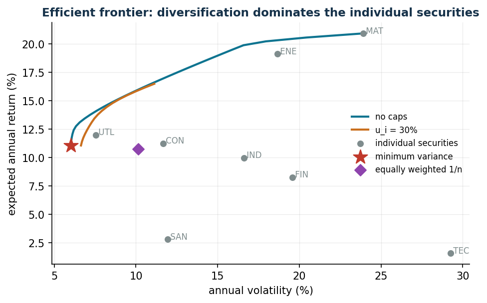
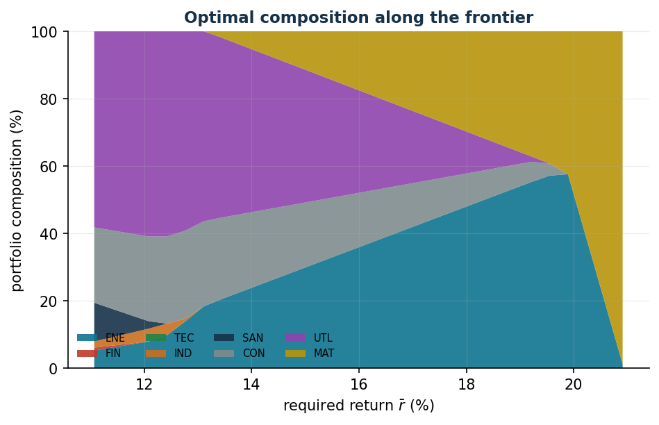
Three messages: (1) the minimum-variance portfolio (volatility 6%) is much less risky than the best individual asset (UTL, 7.5%) while still returning 11%; (2) the equally weighted \(1/n\) portfolio — the "I know nothing" strategy — is clearly dominated: the same region of return but almost twice the volatility; (3) the cap \(u_i = 30\%\) cuts off the upper part of the frontier — the cost of the mandate constraints can be seen as the distance between the two curves.
Sensitivity
r_min =  6%: vol 6.03%   (constraint NOT active: same as min variance)
r_min =  8%: vol 6.03%   (same)
r_min = 10%: vol 6.03%   (same)
r_min = 12%: vol 6.10%   d(variance)/d(r_min) ~ 0.0221
Up to \(\bar r = 11\%\) the return constraint is inactive: the minimum-variance portfolio already returns 11.06%, hence asking for "at least 8%" costs nothing and the multiplier is zero. Only beyond 11.06% does the constraint bite, and every additional point of return is paid for in variance (multiplier \(\approx 0.022\) at \(\bar r = 12\%\)).
The fragility of the estimates
In the simulated data the asset TEC has a true \(\alpha\) of 11% per year, but over 60 months the estimated return is 1.6%: the noise dominates. The estimates of the expected returns are far more unstable than those of the covariances, and optimized portfolios chase the estimation errors. Remedies: the constraints \(u_i\), shrinkage of the estimates, or optimizing risk only (minimum variance).
Code
The complete script of the chapter — data, model, solution, sensitivity and figures —
is python/lab06_markowitz.py
(reproducible with python3 python/lab06_markowitz.py from the python/ folder).
The same code is also available as a notebook — notebooks/lab06_markowitz.ipynb — which opens in Colab from the badge at the top of the page and runs in the browser, with nothing to install.
Show the full script — lab06_markowitz.py
"""Chapter 6 — Markowitz portfolio (convex QP).

Case study: 8 securities (sector ETFs), 60 monthly returns simulated with a
one-factor market model + idiosyncratic noise.

Contents:
  1. Estimation of mu and Q from the historical data
  2. Global minimum-variance portfolio and portfolio with a minimum return
  3. Efficient frontier and composition along the frontier
  4. Effect of the per-security upper bounds (u_i)
"""
import gurobipy as gp
import numpy as np
import pandas as pd
from gurobipy import GRB

from stile import (ARANCIO, CICLO, GRIGIO, ROSSO, TEAL, intestazione, plt, salva_dat,
                   salva_dati, salva_figura)

rng = np.random.default_rng(42)

# ----------------------------------------------------------------------
# 1. DATA: 60 months of simulated returns (one-factor model)
# ----------------------------------------------------------------------
titoli = ["ENE", "FIN", "TEC", "IND", "SAN", "CON", "UTL", "MAT"]
n, T = len(titoli), 60
beta = np.array([1.1, 1.3, 1.5, 1.0, 0.6, 0.8, 0.4, 1.2])       # market exposure
alfa_ann = np.array([0.05, 0.06, 0.11, 0.05, 0.045, 0.05, 0.035, 0.06])  # excess return
sigma_idio = np.array([0.05, 0.055, 0.07, 0.04, 0.03, 0.035, 0.02, 0.06])  # monthly idio vol

mercato = rng.normal(0.004, 0.035, T)                 # monthly market factor
R = (alfa_ann[None, :] / 12 + np.outer(mercato, beta)
     + rng.normal(0, sigma_idio, (T, n)))             # T x n matrix of returns

rend = pd.DataFrame(R, columns=titoli)
rend.insert(0, "month", range(1, T + 1))
salva_dati(rend, "markowitz_rendimenti")

mu = R.mean(axis=0) * 12                # annualised expected return
Q = np.cov(R.T) * 12                    # annualised covariance
vol = np.sqrt(np.diag(Q))

intestazione("Statistics of the securities (annualised)")
for i, tt in enumerate(titoli):
    print(f"  {tt}: mu = {mu[i]:6.2%}   vol = {vol[i]:6.2%}")


def portafoglio(r_min=None, u=1.0):
    """QP: minimum variance with optional minimum return and per-security cap."""
    m = gp.Model("markowitz")
    m.Params.OutputFlag = 0
    x = m.addVars(n, ub=u, name="x")
    m.addConstr(x.sum() == 1, name="budget")
    if r_min is not None:
        m.addConstr(gp.quicksum(mu[i] * x[i] for i in range(n)) >= r_min, name="return")
    m.setObjective(gp.quicksum(Q[i, j] * x[i] * x[j]
                               for i in range(n) for j in range(n)), GRB.MINIMIZE)
    m.optimize()
    if m.Status != GRB.OPTIMAL:
        return None, None, None
    w = np.array([x[i].X for i in range(n)])
    return w, float(mu @ w), float(np.sqrt(w @ Q @ w))


# ----------------------------------------------------------------------
# 2. NOTABLE PORTFOLIOS
# ----------------------------------------------------------------------
intestazione("Notable portfolios")
w_mv, r_mv, v_mv = portafoglio()
print(f"Global minimum variance : return {r_mv:6.2%}, volatility {v_mv:6.2%}")
w_eq = np.ones(n) / n
print(f"Equally weighted (1/n)  : return {mu @ w_eq:6.2%}, "
      f"volatility {np.sqrt(w_eq @ Q @ w_eq):6.2%}")
r_obb = 0.08
w_8, r_8, v_8 = portafoglio(r_min=r_obb)
print(f"Minimum return 8%       : return {r_8:6.2%}, volatility {v_8:6.2%}")
print("\nComposition (weights > 1%):")
for nome, w in [("min variance", w_mv), ("min return 8%", w_8)]:
    quote = ", ".join(f"{titoli[i]} {w[i]:.1%}" for i in range(n) if w[i] > 0.01)
    print(f"  {nome:>14}: {quote}")

# ----------------------------------------------------------------------
# 3. EFFICIENT FRONTIER (with and without the cap u_i = 30%)
# ----------------------------------------------------------------------
intestazione("Efficient frontier")
r_grid = np.linspace(r_mv, mu.max() * 0.999, 30)
frontiere = {}
for u, etich in [(1.0, "no caps"), (0.30, "u_i = 30%")]:
    punti, composizioni = [], []
    for r in r_grid:
        w, rr, vv = portafoglio(r_min=r, u=u)
        if w is not None:
            punti.append((vv, rr))
            composizioni.append(w)
    frontiere[etich] = (np.array(punti), np.array(composizioni))
    print(f"  frontier '{etich}': {len(punti)} points computed")

pf = frontiere["no caps"][0]
salva_dati(pd.DataFrame({"volatility": pf[:, 0], "return": pf[:, 1]}),
           "markowitz_frontiera")

# ----------------------------------------------------------------------
# 4. FIGURES (pgfplots data + matplotlib preview)
# ----------------------------------------------------------------------
pf_lim = frontiere["u_i = 30%"][0]
salva_dat(pd.DataFrame({"vol": pf[:, 0] * 100, "ret": pf[:, 1] * 100}), "cap06_front_libera")
salva_dat(pd.DataFrame({"vol": pf_lim[:, 0] * 100, "ret": pf_lim[:, 1] * 100}),
          "cap06_front_limiti")
salva_dat(pd.DataFrame({"security": titoli, "vol": vol * 100, "mu": mu * 100}), "cap06_titoli")
salva_dat(pd.DataFrame({
    "name": ["minvar", "equalweight"],
    "vol": [v_mv * 100, float(np.sqrt(w_eq @ Q @ w_eq)) * 100],
    "ret": [r_mv * 100, float(mu @ w_eq) * 100],
}), "cap06_speciali")
punti_sl, comp_sl = frontiere["no caps"]
salva_dat(pd.DataFrame({"ret": punti_sl[:, 1] * 100,
                        **{titoli[i]: comp_sl[:, i] * 100 for i in range(n)}}),
          "cap06_composizione")

fig, ax = plt.subplots()
for (etich, (punti, _)), colore in zip(frontiere.items(), [TEAL, ARANCIO]):
    ax.plot(punti[:, 0] * 100, punti[:, 1] * 100, "-", color=colore, lw=2, label=etich)
ax.scatter(vol * 100, mu * 100, color=GRIGIO, s=28, zorder=3, label="individual securities")
for i, tt in enumerate(titoli):
    ax.annotate(" " + tt, (vol[i] * 100, mu[i] * 100), fontsize=8, color=GRIGIO)
ax.scatter([v_mv * 100], [r_mv * 100], marker="*", s=200, color=ROSSO, zorder=4,
           label="minimum variance")
ax.scatter([np.sqrt(w_eq @ Q @ w_eq) * 100], [mu @ w_eq * 100], marker="D", s=60,
           color="#8E44AD", zorder=4, label="equally weighted 1/n")
ax.set_xlabel("annual volatility (%)")
ax.set_ylabel("expected annual return (%)")
ax.set_title("Efficient frontier: diversification dominates the individual securities")
ax.legend(fontsize=8)
salva_figura(fig, "cap06_frontiera")

punti, comp = frontiere["no caps"]
fig, ax = plt.subplots()
ax.stackplot(punti[:, 1] * 100, (comp.T * 100), labels=titoli, colors=CICLO, alpha=0.9)
ax.set_xlabel("required return $\\bar r$ (%)")
ax.set_ylabel("portfolio composition (%)")
ax.set_title("Optimal composition along the frontier")
ax.legend(fontsize=7, ncol=4, loc="lower left")
ax.set_ylim(0, 100)
salva_figura(fig, "cap06_composizione")

# sensitivity: price of the return constraint (multiplier ~ slope of the frontier)
intestazione("Sensitivity: cost (in variance) of the required return")
for r in [0.06, 0.08, 0.10, 0.12]:
    w, rr, vv = portafoglio(r_min=r)
    if w is None:
        print(f"  r_min = {r:.0%}: infeasible (beyond the maximum return)")
        continue
    eps = 0.002
    w2, _, vv2 = portafoglio(r_min=r + eps)
    pend = (vv2**2 - vv**2) / eps if w2 is not None else float("nan")
    print(f"  r_min = {r:5.1%}: vol {vv:6.2%}  |  d(variance)/d(r_min) ~ {pend:7.4f}")

print("\nDone: chapter 6.")
Exercises
- Two assets with \(\rho = 0.5\): is diversification still worthwhile? (\(x_1 = 6/7\), vol 19.6%)
- Frontiers with \(u = 1\), \(0.3\), \(0.2\): maximum return 20.9% / 16.7% / 14.7%.
- Run again with a different seed: how much do the compositions change?
- Minimum tracking error with return ≥ 12% (TE = 1.1% per year).
- Quadratic transaction costs starting from the equally weighted portfolio.