Arbitrage and arbitrage-free pricing
Lecture notes (PDF) · Chapter slides (PDF)
Class: LP · Script: python/lab14_arbitrage.py

An arbitrage is a strategy that creates money out of nothing: it collects cash today with no risk of a loss tomorrow (type A), or it costs nothing today and can only make money (type B). Detecting one is an LP; duality — shadow prices, complementary slackness, strong duality — becomes the theory of pricing. It is the cleanest application of the primal-dual pair in the whole lab.
The model
One-stage market: today we buy or sell at the prices \(s^0_i\); tomorrow one out of \(m\) states of the world occurs and security \(i\) pays \(s^1_{ij}\). Security \(0\) is risk-free: it costs \(1\) and pays \(R = 1 + r\) in every state. Variables: the positions \(x_i\) (free: buying or short selling).
The null portfolio is feasible, hence the optimum is always \(\le 0\). If the optimum is \(< 0\) there is a type A arbitrage and, the constraints being homogeneous, the model is unbounded: for a finite certificate one adds the normalization \(\sum_i s^0_i x_i \ge -1\) ("collect at most 1 today").
Duality is pricing
With the duality rules (minimization primal): every state generates a \(p_j \ge 0\), every free position a dual equality constraint:
From the constraint of security 0: \(\sum_j p_j = 1/R\), hence \(q_j = R\, p_j\) are risk-neutral probabilities and
today's price is the discounted expected value of tomorrow's payoffs under \(q\).
Fundamental theorem of asset pricing
There is no arbitrage (neither type A nor type B) if and only if there exists a risk-neutral measure with \(q_j > 0\) for every state. It is strong duality (no type A ⇒ the dual is feasible) plus complementary slackness (no type B ⇒ there exists a measure with \(q > 0\)).
Case study
Three states, \(R = 1{,}04\), two risky securities with payoffs \((10, 15, 13)\) and
\((30, 15, 25)\) — data in data/arbitraggio_payoff.csv.
Prices (6, 20):      without normalization: UNBOUNDED (type A)
  normalized: optimum -1  ->  collect 1 today, payoff (0; 0; 0.20) >= 0
  by hand: (-27, 1, 1) collects 1 with payoff (11.92; 1.92; 9.92)
Prices (13, 18.69):  optimum 0, no arbitrage
  duals of the state constraints p* = (0.2846; 0.6769; 0)
  q = R p*             = (0.296;  0.704;  0)   sum 1
  pricing check: s0 = (1; 13; 18.6923) reproduced exactly
The duals price: every security, even a new one, is worth its discounted expected payoff under \(q\). The value \(q_3 = 0\) signals that state 3 is not needed to price these securities — and it is the reason why the theorem requires \(q > 0\): with \(q_3 = 0\) a latent type B arbitrage on state 3 remains.
Sensitivity: the interval of consistent prices
With only securities 0 and 1 quoted (1 and 13), the prices of security 2 that do not create arbitrage form an interval, computed with two LPs (min and max of \(\sum_j s^1_{2j} p_j\) over the consistent measures):
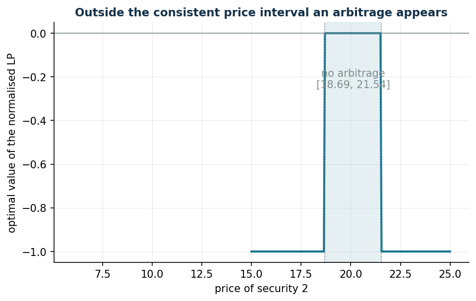
Inside the interval the value of the normalized LP is 0 (consistent prices); outside it drops to −1: an arbitrage exists, in one direction or the other.
Pricing a new security. A call on security 1 with strike 12 pays \((0, 3, 1)\):
- complete market (securities 0, 1, 2 quoted): a unique measure, a unique price \(2{,}0308\);
- incomplete market (only 0 and 1): infinitely many consistent measures, price in \([1{,}4615,\; 2{,}0308]\) — outside that interval anyone could build an arbitrage by combining the call and the quoted securities.
The same code is also available as a notebook — notebooks/lab14_arbitrage.ipynb — which opens in Colab from the badge at the top of the page and runs in the browser, with nothing to install.
Show the full script — lab14_arbitrage.py
"""Chapter 14 — Arbitrage and arbitrage-free pricing (LP).

Case study: a one-period market with 3 states of the world, one risk-free
security (gross return R = 1.04) and 2 risky securities.

Contents:
  1. Detecting an arbitrage (normalised LP): prices (6, 20) -> a gain of 1 today
  2. Consistent prices (13, 18.6923): optimum 0 and risk-neutral probabilities
     from the duals of the state constraints
  3. Arbitrage-free price interval for security 2 (two LPs + a grid)
  4. Pricing a call: complete market (unique price) vs incomplete (range)
"""
import gurobipy as gp
import numpy as np
import pandas as pd
from gurobipy import GRB

from stile import ARANCIO, GRIGIO, ROSSO, TEAL, intestazione, plt, salva_dat, salva_dati, salva_figura

# ----------------------------------------------------------------------
# 1. DATA: payoff s1[i][j] of security i in state j; security 0 is risk free
# ----------------------------------------------------------------------
r = 0.04
R = 1 + r                                     # gross return of security 0
s1 = np.array([[R, R, R],                     # security 0
               [10.0, 15.0, 13.0],            # security 1
               [30.0, 15.0, 25.0]])           # security 2
n1, n_stati = s1.shape                        # 3 securities (0,1,2), 3 states

salva_dati(pd.DataFrame(s1, columns=[f"state_{j+1}" for j in range(n_stati)],
                        index=["security_0", "security_1", "security_2"]).reset_index(names="security"),
           "arbitraggio_payoff")


def lp_arbitraggio(s0, normalizza=True):
    """min sum s0_i x_i  subject to  payoff >= 0 in every state (x free).

    With `normalizza` it adds  sum s0_i x_i >= -1  (today's proceeds at most 1):
    without it, in the presence of a type-A arbitrage the model is unbounded."""
    m = gp.Model("arbitrage")
    m.Params.OutputFlag = 0
    m.Params.DualReductions = 0               # distinguishes UNBOUNDED from INFEASIBLE
    x = m.addVars(n1, lb=-GRB.INFINITY, name="x")
    v_stato = m.addConstrs(
        (gp.quicksum(s1[i, j] * x[i] for i in range(n1)) >= 0
         for j in range(n_stati)), name="state")
    if normalizza:
        m.addConstr(gp.quicksum(s0[i] * x[i] for i in range(n1)) >= -1,
                    name="normalisation")
    m.setObjective(gp.quicksum(s0[i] * x[i] for i in range(n1)), GRB.MINIMIZE)
    m.optimize()
    return m, x, v_stato


# ----------------------------------------------------------------------
# 2. DETECTING AN ARBITRAGE: prices (1, 6, 20)
# ----------------------------------------------------------------------
intestazione("Prices (6, 20): is there an arbitrage?")
s0_arb = np.array([1.0, 6.0, 20.0])
m_nb, _, _ = lp_arbitraggio(s0_arb, normalizza=False)
print(f"LP without normalisation: status {m_nb.Status} "
      f"({'UNBOUNDED: type-A arbitrage' if m_nb.Status == GRB.UNBOUNDED else 'optimal'})")
m_a, x_a, _ = lp_arbitraggio(s0_arb)
print(f"Normalised LP: optimal value {m_a.ObjVal:.4f} "
      f"(= proceeds of 1 today with no risk at all)")
print("Strategy:", {f"x{i}": round(x_a[i].X, 4) for i in range(n1)})
payoff = s1.T @ np.array([x_a[i].X for i in range(n1)])
print("Payoff in the three states:", np.round(payoff, 4), "(all >= 0)")
# the "by hand" strategy of the chapter: (-27, 1, 1)
x_libro = np.array([-27.0, 1.0, 1.0])
print(f"Strategy (-27, 1, 1): cost {s0_arb @ x_libro:.0f}, "
      f"payoff {np.round(s1.T @ x_libro, 2)} (equivalent, on a different scale)")

# ----------------------------------------------------------------------
# 3. CONSISTENT PRICES: optimum 0 and risk-neutral probabilities
# ----------------------------------------------------------------------
intestazione("Prices (13, 18.6923): no arbitrage and pricing")
s0_ok = np.array([1.0, 13.0, 18.692308])
m_b, x_b, v_stato = lp_arbitraggio(s0_ok, normalizza=False)
print(f"Optimal value: {m_b.ObjVal:.4f}  (null strategy: no arbitrage)")
p = np.array([v_stato[j].Pi for j in range(n_stati)])
q = R * p
print(f"Duals of the state constraints p* = {np.round(p, 4)}")
print(f"Risk-neutral probabilities q = R p* = {np.round(q, 4)} "
      f"(sum = {q.sum():.4f})")
print("Pricing check: s0_i = sum_j p_j s1_ij =",
      np.round(s1 @ p, 4))

# ----------------------------------------------------------------------
# 4. ARBITRAGE-FREE PRICE INTERVAL FOR SECURITY 2
# ----------------------------------------------------------------------
intestazione("Arbitrage-free price interval for security 2")


def bound_prezzo(payoff_nuovo, quotati, senso):
    """min/max of sum_j p_j payoff_j over the measures p >= 0 consistent with the quoted ones."""
    d = gp.Model("pricing")
    d.Params.OutputFlag = 0
    pp = d.addVars(n_stati, name="p")
    for i, prezzo in quotati:
        d.addConstr(gp.quicksum(s1[i, j] * pp[j] for j in range(n_stati)) == prezzo)
    d.setObjective(gp.quicksum(payoff_nuovo[j] * pp[j] for j in range(n_stati)), senso)
    d.optimize()
    assert d.Status == GRB.OPTIMAL
    return d.ObjVal


quotati_01 = [(0, 1.0), (1, 13.0)]
lo = bound_prezzo(s1[2], quotati_01, GRB.MINIMIZE)
hi = bound_prezzo(s1[2], quotati_01, GRB.MAXIMIZE)
print(f"With security 0 and security 1 quoted (1 and 13): the price of security 2 "
      f"is arbitrage free in [{lo:.4f}, {hi:.4f}]")

griglia = np.linspace(15, 25, 201)
valori = []
for prezzo2 in griglia:
    mg, _, _ = lp_arbitraggio(np.array([1.0, 13.0, prezzo2]))
    valori.append(mg.ObjVal)
curva = pd.DataFrame({"price_security2": griglia, "lp_value": valori})
salva_dati(curva, "arbitraggio_curva_prezzo")
salva_dat(curva, "cap14_arbitraggio_curva")
print(f"Grid {griglia[0]:.0f}..{griglia[-1]:.0f}: LP value = 0 only inside "
      f"the interval, negative outside (arbitrage)")

# ----------------------------------------------------------------------
# 5. PRICING A CALL ON SECURITY 1 (STRIKE 12)
# ----------------------------------------------------------------------
intestazione("Pricing a call on security 1, strike 12")
call = np.maximum(s1[1] - 12.0, 0.0)
print("Payoff of the call in the three states:", call)
quotati_012 = [(0, 1.0), (1, 13.0), (2, 18.692308)]
lo_c = bound_prezzo(call, quotati_012, GRB.MINIMIZE)
hi_c = bound_prezzo(call, quotati_012, GRB.MAXIMIZE)
print(f"Complete market (securities 0, 1, 2 quoted): unique price "
      f"[{lo_c:.4f}, {hi_c:.4f}]")
lo_i = bound_prezzo(call, quotati_01, GRB.MINIMIZE)
hi_i = bound_prezzo(call, quotati_01, GRB.MAXIMIZE)
print(f"Incomplete market (only securities 0 and 1): interval   "
      f"[{lo_i:.4f}, {hi_i:.4f}]")

# ----------------------------------------------------------------------
# 6. FIGURE: arbitrage gain as the price of security 2 varies
# ----------------------------------------------------------------------
fig, ax = plt.subplots()
ax.plot(curva["price_security2"], curva["lp_value"], color=TEAL, lw=2)
ax.axvspan(lo, hi, color=TEAL, alpha=0.10)
ax.axvline(lo, color=GRIGIO, ls=":", lw=1)
ax.axvline(hi, color=GRIGIO, ls=":", lw=1)
ax.axhline(0, color=GRIGIO, lw=0.8)
ax.annotate(f"no arbitrage\n[{lo:.2f}, {hi:.2f}]",
            ((lo + hi) / 2, -0.25), ha="center", color=GRIGIO)
ax.plot([6], [0], alpha=0)  # noop
ax.set_xlabel("price of security 2")
ax.set_ylabel("optimal value of the normalised LP")
ax.set_title("Outside the consistent price interval an arbitrage appears")
salva_figura(fig, "cap14_arbitraggio_curva")

print("\nDone: chapter 14 (arbitrage).")
Exercises
- With prices \((6, 20)\), find a strategy that collects 5 today with no risk tomorrow.
- Set the price of security 2 at the upper endpoint \(21{,}5385\): check that the optimum is 0 and compute the pricing measure. What happens at \(21{,}60\)?
- In the complete market, price a call on security 2 with strike 20 and check the price with the risk-neutral probabilities.