Smart charging of electric vehicles
Lecture notes (PDF) · Chapter slides (PDF)
Class: LP / convex QP · Script: python/lab10_ev_charging.py

A fleet must be fully charged by the morning by exploiting the cheap hours — but if all the vehicles charge together, the peak draw explodes. A problem that seems to require on/off variables and instead is a pure LP: the real decision — how much power — is continuous.
The problem in words. We decide the power \(x_{vt}\) for each vehicle and hour. The objective: minimum energy expenditure. The constraints: the energy required before departure, charging only while plugged in and below the power of the charger, total draw below the power of the meter.
Model
Data (input of the model).
| Symbol | Type | Meaning |
|---|---|---|
| \(n\) | \(\in \mathbb{Z}_{\ge 1}\) | number of vehicles, indexed by \(v \in \{1, 2, \dots, n\}\) |
| \(m\) | \(\in \mathbb{Z}_{\ge 1}\) | number of hourly intervals, indexed by \(t \in \{1, 2, \dots, m\}\), of duration \(\Delta t\) (here \(\Delta t = 1\) h) |
| \(\pi_t\) | \(\in \mathbb{Q}_{\ge 0}\) | energy price in hour \(t\) (€/kWh) |
| \(a_{vt}\) | \(\in \{0, 1\}\) | observed datum: \(1\) if vehicle \(v\) is plugged in during hour \(t\), \(0\) otherwise |
| \(e_v\) | \(\in \mathbb{Q}_{> 0}\) | energy required by vehicle \(v\) before departure (kWh) |
| \(\bar p_v\) | \(\in \mathbb{Q}_{> 0}\) | maximum charging power of vehicle \(v\) (kW) |
| \(b_t\) | \(\in \mathbb{Q}_{\ge 0}\) | base load of the building in hour \(t\) (kW) |
| \(k\) | \(\in \mathbb{Q}_{> 0}\) | maximum power that can be drawn from the meter (kW) |
| \(\eta\) | \(\in \mathbb{Q},\ 0 < \eta \le 1\) | charging efficiency |
Decision variables. We introduce the following \(n\,m\) non-negative variables:
Using these variables, an LP model for the problem is the following:
Description of the objective function and of the constraints:
- the linear objective function minimizes the energy expenditure of the night: the power \(x_{vt}\) delivered for the duration \(\Delta t\) costs \(\pi_t\, \Delta t\, x_{vt}\) euros;
- the linear energy constraints ensure that every vehicle receives all the energy it requires before departure; the efficiency \(\eta\) stands on the left: of the energy that is drawn, only the fraction \(\eta\) ends up in the battery (\(n\) linear constraints);
- the linear grid constraints impose that the overall draw (charging plus base load) never exceeds the power of the meter: these are the constraints that couple the vehicles to each other (\(m\) linear constraints);
- the linear power constraints limit the power of every vehicle to that of its charger and set it to zero in the hours in which the vehicle is absent (\(a_{vt} = 0\)): availability is a datum, not a decision, and this is why no binary variables are needed (\(n\,m\) linear constraints);
- the non-negativity constraints on \(x_{vt}\) define the variables of the model.
Variants: peak shaving (\(\min z\) with \(\sum_{v=1}^{n} x_{vt} + b_t \le z\) for every \(t \in \{1, 2, \dots, m\}\)); smooth profile (QP with \(\gamma \sum_{t=2}^{m} (z_t - z_{t-1})^2\)); multi-objective cost \(+\,\rho\,z\). The energy constraint is written as \(\ge\) because charging more than necessary is allowed but never worthwhile (the price is positive): at the optimum it holds with equality.
Worked example by hand (1 vehicle, 2 hours)
\(e = 10\) kWh (\(\eta = 1\)), prices \(\pi_1 = 0{,}10\) and \(\pi_2 = 0{,}20\) €/kWh, \(\bar p = 8\) kW: we charge 8 kWh in the cheap hour and 2 in the expensive one (cost \(8 \cdot 0{,}10 + 2 \cdot 0{,}20 = 1{,}20\) €). Shadow price of the energy requirement = 0.20 €/kWh (the price of the marginal hour); shadow price of the power limit in hour 1 = 0.10 €/kW. With \(\bar p = 12\): everything in the cheap hour, cost 1.00 €, dual of the requirement 0.10 and dual of the power 0 (constraint not active).
Case study
Six vans with different night windows, meter \(k = 120\) kW, \(\eta = 0{,}95\).
Minimum cost   : 20.36 EUR/night   peak draw 103.4 kW (limit 120)
Peak shaving   : minimum possible peak 68.0 kW
Shadow prices of the energy requirement (EUR/kWh):
  V1 0.0947   V2 0.0842   V3 0.0842   V4 0.0947   V5 0.0947   V6 0.0842
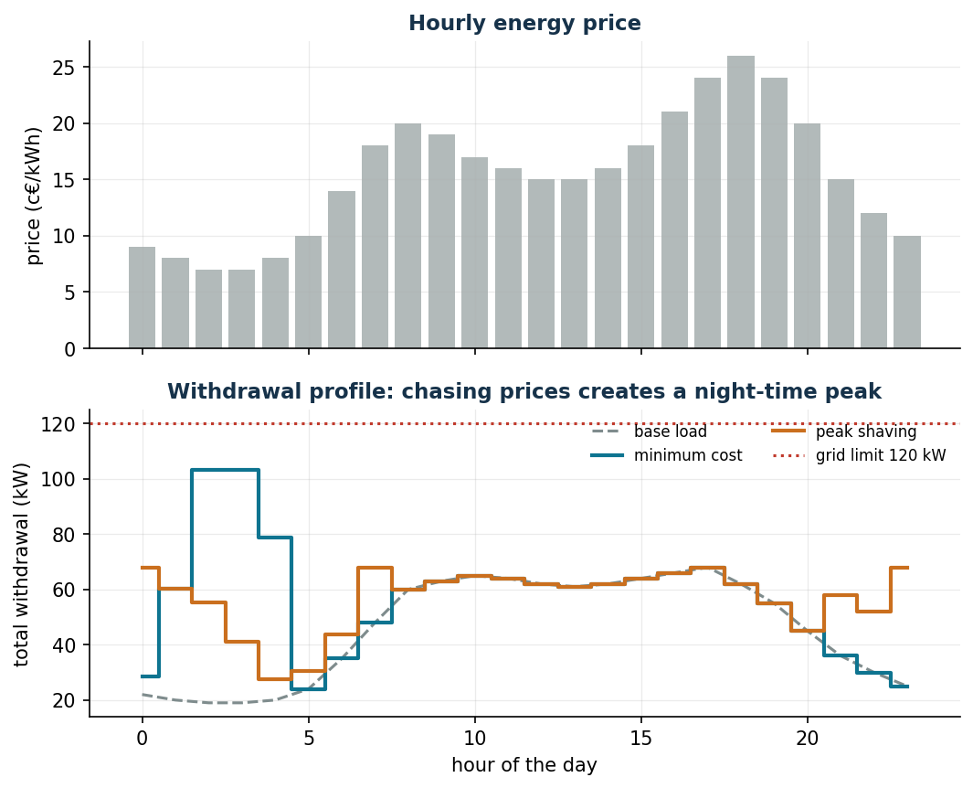
The shadow prices of the energy requirement are equal to \(0{,}0842 = 0{,}08/\eta\) or \(0{,}0947 = 0{,}09/\eta\): they are the prices of the marginal hours of each vehicle (the cheapest hour still free within its window), corrected for the efficiency. V2, V3 and V6 have windows that cover the hours at \(0{,}08\); V1, V4 and V5 arrive late or leave early and their marginal hour costs \(0{,}09\). One additional kWh of requirement therefore costs between 8.4 and 9.5 cents depending on the vehicle.
Sensitivity
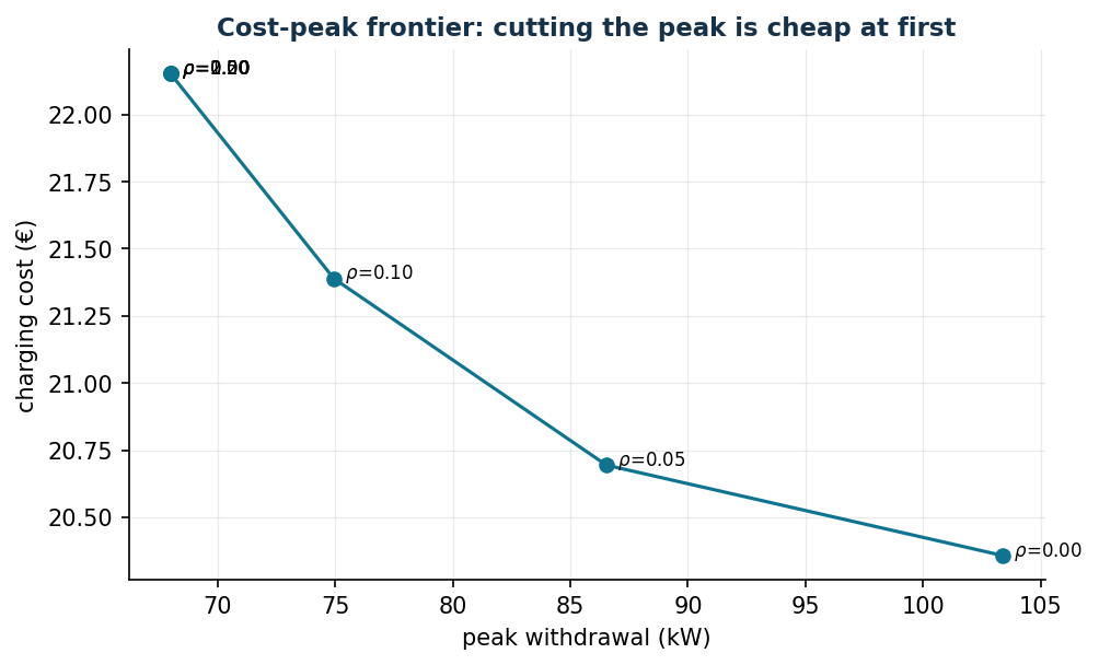
Trade-off cost + rho*peak:
  rho = 0.00: cost 20.36  peak 103.4     rho = 0.20: cost 22.15  peak 68.0
  rho = 0.05: cost 20.69  peak  86.5     rho = 0.50: cost 22.15  peak 68.0
  rho = 0.10: cost 21.39  peak  74.9
Meter capacity:
  k = 60, 65 kW: INFEASIBLE     k = 80: 21.09     k = 120: 20.36
  k = 70 kW    : 21.93          k = 90: 20.63
Cutting the peak from 103 to 75 kW (−28%) costs only one euro per night; getting down to 68 kW costs less than two. The pure minimax (peak 68) without the cost term would spend 27.79 €: the trade-off with \(\rho = 0{,}2\) achieves the same peak at 22.15 € — never optimize a single objective when there are two of them.
An instructive bug (which really happened)
In the constraint quicksum(x) + base[t] <= C Gurobi moves the constant into the
right-hand side: the stored RHS is C - base[t]. Whoever writes v.RHS = newC
is relaxing the wrong constraint. When a sensitivity analysis changes nothing,
suspect your own code before suspecting the model.
Code
The complete script of the chapter — data, model, solution, sensitivity and figures —
is python/lab10_ev_charging.py
(reproducible with python3 python/lab10_ev_charging.py from the python/ folder).
The same code is also available as a notebook — notebooks/lab10_ev_charging.ipynb — which opens in Colab from the badge at the top of the page and runs in the browser, with nothing to install.
Show the full script — lab10_ev_charging.py
"""Chapter 10 — Smart charging of electric vehicles (LP / convex QP).

Case study: a company depot with 6 electric vans to be charged overnight;
hourly energy prices; base load of the building.

Contents:
  1. Minimum-cost LP: charging chases the cheap hours
  2. Peak shaving: minimise the peak withdrawal (minimax)
  3. Smooth profile (QP) and multi-objective cost-peak comparison
  4. Shadow prices: grid capacity and energy requirement
"""
import gurobipy as gp
import numpy as np
import pandas as pd
from gurobipy import GRB

from stile import (ARANCIO, GRIGIO, ROSSO, TEAL, intestazione, plt, salva_dat, salva_dati,
                   salva_figura)

# ----------------------------------------------------------------------
# 1. DATA
# ----------------------------------------------------------------------
ore = list(range(24))                      # hour t = [t, t+1)
# price €/kWh: high during the day and in the evening peak, low at night
prezzo = np.array([0.09, 0.08, 0.07, 0.07, 0.08, 0.10, 0.14, 0.18, 0.20, 0.19,
                   0.17, 0.16, 0.15, 0.15, 0.16, 0.18, 0.21, 0.24, 0.26, 0.24,
                   0.20, 0.15, 0.12, 0.10])
# base load of the building (kW)
base = np.array([22, 20, 19, 19, 20, 24, 35, 48, 60, 63, 65, 64,
                 62, 61, 62, 64, 66, 68, 62, 55, 45, 36, 30, 25], dtype=float)

veicoli = [f"V{k}" for k in range(1, 7)]
# (arrival hour, departure hour, required energy kWh, max power kW)
flotta = {
    "V1": (18, 7, 46, 11), "V2": (19, 6, 38, 11), "V3": (20, 8, 55, 22),
    "V4": (17, 6, 30, 7.4), "V5": (21, 7, 42, 11), "V6": (22, 8, 50, 22),
}
eta = 0.95            # charging efficiency
C_rete = 120.0        # maximum power that can be drawn from the meter (kW)

disp = {(v, t): 1 if (flotta[v][0] <= t or t < flotta[v][1]) else 0
        for v in veicoli for t in ore}      # windows that straddle midnight

salva_dati(pd.DataFrame({"hour": ore, "price": prezzo, "base_load": base}), "ev_prezzi_base")
salva_dati(pd.DataFrame([(v, *flotta[v]) for v in veicoli],
                        columns=["vehicle", "arrival", "departure", "energy_kWh", "pmax_kW"]),
           "ev_flotta")


def costruisci():
    m = gp.Model("ev_charging")
    m.Params.OutputFlag = 0
    x = m.addVars(veicoli, ore, name="x")       # charging power (kW)
    for v in veicoli:
        for t in ore:
            x[v, t].UB = flotta[v][3] * disp[v, t]     # 0 if not plugged in
    v_ene = m.addConstrs((eta * gp.quicksum(x[v, t] for t in ore) >= flotta[v][2]
                          for v in veicoli), name="energy")
    v_rete = m.addConstrs((gp.quicksum(x[v, t] for v in veicoli) + base[t] <= C_rete
                           for t in ore), name="grid")
    return m, x, v_ene, v_rete


def profilo(x):
    return np.array([sum(x[v, t].X for v in veicoli) for t in ore])


# ----------------------------------------------------------------------
# 2. MINIMUM-COST LP
# ----------------------------------------------------------------------
intestazione("LP: minimum energy cost")
m, x, v_ene, v_rete = costruisci()
m.setObjective(gp.quicksum(prezzo[t] * x[v, t] for v in veicoli for t in ore), GRB.MINIMIZE)
m.optimize()
assert m.Status == GRB.OPTIMAL
prof_costo = profilo(x)
costo_min = m.ObjVal
picco_costo = (prof_costo + base).max()
print(f"Charging cost: {costo_min:.2f} €   peak withdrawal: {picco_costo:.1f} kW "
      f"(limit {C_rete:.0f})")
print("\nShadow prices of the energy requirement (marginal cost of 1 more kWh per vehicle):")
for v in veicoli:
    print(f"  {v}: {v_ene[v].Pi:.4f} €/kWh")

# ----------------------------------------------------------------------
# 3. PEAK SHAVING (minimax) and SMOOTH PROFILE (QP)
# ----------------------------------------------------------------------
intestazione("Peak shaving: minimise the peak withdrawal")
mp, xp, _, _ = costruisci()
z = mp.addVar(name="peak")
mp.addConstrs((gp.quicksum(xp[v, t] for v in veicoli) + base[t] <= z for t in ore),
              name="peak_def")
mp.setObjective(z, GRB.MINIMIZE)
mp.optimize()
prof_picco = profilo(xp)
costo_picco = sum(prezzo[t] * prof_picco[t] for t in ore)
print(f"Lowest achievable peak: {mp.ObjVal:.1f} kW   cost: {costo_picco:.2f} € "
      f"(+{costo_picco - costo_min:.2f} € with respect to the minimum cost)")

intestazione("Trade-off: cost + rho · peak")
compromessi = []
for rho in [0, 0.05, 0.1, 0.2, 0.5, 1.0, 2.0]:
    mc, xc, _, _ = costruisci()
    zc = mc.addVar(name="peak")
    mc.addConstrs((gp.quicksum(xc[v, t] for v in veicoli) + base[t] <= zc for t in ore))
    mc.setObjective(gp.quicksum(prezzo[t] * xc[v, t] for v in veicoli for t in ore)
                    + rho * zc, GRB.MINIMIZE)
    mc.optimize()
    cc = sum(prezzo[t] * xc[v, t].X for v in veicoli for t in ore)
    compromessi.append((rho, cc, zc.X))
    print(f"  rho = {rho:4.2f}: cost {cc:6.2f} €, peak {zc.X:6.1f} kW")
salva_dati(pd.DataFrame(compromessi, columns=["rho", "cost", "peak"]), "ev_compromessi")

# ----------------------------------------------------------------------
# 4. SENSITIVITY: capacity of the meter
# ----------------------------------------------------------------------
intestazione("Sensitivity: capacity of the grid connection")
# careful: in the constraint "sum x + base[t] <= C" Gurobi moves the constant base[t]
# into the right-hand side; the stored RHS is C - base[t], so it must be updated like this:
for CC in [60, 65, 70, 80, 90, 120]:
    ms, xs_, _, vr = costruisci()
    for t in ore:
        vr[t].RHS = CC - base[t]
    ms.setObjective(gp.quicksum(prezzo[t] * xs_[v, t] for v in veicoli for t in ore),
                    GRB.MINIMIZE)
    ms.optimize()
    esito = f"cost {ms.ObjVal:6.2f} €" if ms.Status == GRB.OPTIMAL else "INFEASIBLE"
    print(f"  C_grid = {CC:3d} kW: {esito}")

# ----------------------------------------------------------------------
# 5. FIGURES (pgfplots data + matplotlib preview)
# ----------------------------------------------------------------------
salva_dat(pd.DataFrame({"hour": ore, "price_cent": prezzo * 100, "base": base,
                        "totcost": base + prof_costo, "totpeak": base + prof_picco}),
          "cap10_profili")
salva_dat(pd.DataFrame(compromessi, columns=["rho", "cost", "peak"]), "cap10_frontiera")

fig, (ax1, ax2) = plt.subplots(2, 1, figsize=(8.2, 6.4), sharex=True)
ax1.bar(ore, prezzo * 100, color=GRIGIO, alpha=0.6)
ax1.set_ylabel("price (c€/kWh)")
ax1.set_title("Hourly energy price")
ax2.plot(ore, base, color=GRIGIO, ls="--", label="base load")
ax2.plot(ore, base + prof_costo, color=TEAL, lw=2, drawstyle="steps-mid",
         label="minimum cost")
ax2.plot(ore, base + prof_picco, color=ARANCIO, lw=2, drawstyle="steps-mid",
         label="peak shaving")
ax2.axhline(C_rete, color=ROSSO, ls=":", label=f"grid limit {C_rete:.0f} kW")
ax2.set_xlabel("hour of the day"); ax2.set_ylabel("total withdrawal (kW)")
ax2.set_title("Withdrawal profile: chasing prices creates a night-time peak")
ax2.legend(fontsize=8, ncol=2)
salva_figura(fig, "cap10_profili")

comp = pd.DataFrame(compromessi, columns=["rho", "cost", "peak"])
fig, ax = plt.subplots()
ax.plot(comp["peak"], comp["cost"], "-o", color=TEAL)
for _, r in comp.iterrows():
    ax.annotate(f"  $\\rho$={r['rho']:.2f}", (r["peak"], r["cost"]), fontsize=8)
ax.set_xlabel("peak withdrawal (kW)")
ax.set_ylabel("charging cost (€)")
ax.set_title("Cost-peak frontier: cutting the peak is cheap at first")
salva_figura(fig, "cap10_frontiera")

print("\nDone: chapter 10.")
Exercises
- \(e_1: 46 \to 47\) kWh: cost \(+0{,}0947 = 0{,}09/0{,}95\) (verified).
- V3 arrives at 23: how do cost and peak change?
- Smooth profile QP with \(\gamma \sum_t (z_t - z_{t-1})^2\).
- Cost-emissions frontier with an hourly carbon intensity \(g_t\).
- Minimum feasible capacity by bisection: \(\tilde k = 68\) kW.