Service capacity and waiting times
Lecture notes (PDF) · Chapter slides (PDF)
Class: convex NLP (M/M/1 queue) · Script: python/lab11_queues.py

How much capacity should be assigned to a call centre, a service desk, a cloud service? More capacity costs money; too little capacity makes the waiting times explode. The central message, counter-intuitive for anyone who reasons "by efficiency": the optimal utilization is not 100%.
The problem in words. We decide the capacity \(\mu\). The objective: the cost of capacity plus the value of the customers' time in the system. The constraint: stability, \(\mu > \lambda\).
Model
We use the simplest queueing model, the M/M/1: Markovian arrivals (a Poisson process), Markovian service times (exponential) and one server. What is new here is treating the capacity \(\mu\) as an optimization variable.
Data (input of the model).
| Symbol | Type | Meaning |
|---|---|---|
| \(\lambda\) | \(\in \mathbb{Q}_{> 0}\) | mean arrival rate of the customers (requests/hour) |
| \(c\) | \(\in \mathbb{Q}_{> 0}\) | cost of one unit of capacity (€ per unit of \(\mu\) per hour) |
| \(h\) | \(\in \mathbb{Q}_{> 0}\) | value of one hour spent by a customer in the system (€) |
Decision variable and derived quantities. We introduce one continuous variable:
with the stability requirement \(\mu > \lambda\). From M/M/1 queueing theory we obtain the mean time in the system \(w(\mu) = 1/(\mu - \lambda)\) (in the literature: \(W\)) and the mean number of customers in the system \(l(\mu) = \lambda/(\mu - \lambda)\) (Little's law; in the literature: \(L\)).
Using this variable, the model for the problem is the following:
Description of the objective function and of the constraint:
- the objective function is the sum of two terms: the first, \(c\,\mu\), buys the capacity; the second, \(h \cdot l(\mu)\), monetizes the total time the customers spend in the system; it is convex on \((\lambda, +\infty)\);
- the stability constraint defines the variable and guarantees that the queue does not diverge: with \(\mu \le \lambda\) the line grows without bound.
Setting the derivative of the objective to zero gives the closed-form solution:
"Capacity = demand + safety stock": the margin \(\sqrt{h\lambda/c}\) grows with the value of the customers' time, decreases with the cost of capacity, and scales like \(\sqrt\lambda\) (economies of scale in the buffer → pooling).
Worked example by hand
\(\lambda = 8\)/h, \(c = 2\) €, \(h = 4\) €/h: \(\tilde\mu = 8 + \sqrt{4 \cdot 8/2} = 12\) customers/hour, \(\rho = 8/12 = 66{,}7\%\), \(w = 1/(12 - 8) = 15\) min, cost \(2 \cdot 12 + 4 \cdot 8/4 = 32\) €/h. "Cutting the waste" down to \(\mu = 9\) (\(\rho = 89\%\)) would cost \(18 + 32 = 50\) €/h: the apparent waste of 33% of unused capacity is exactly what keeps the queues short.
Case study
\(\lambda = 42\) requests/hour, \(c = 3\) €, \(h = 1{,}5\) €.
Analytical: mu* = 42 + sqrt(1.5*42/3) = 46.583   cost 153.495 EUR/h
Gurobi    : mu* = 46.582 (bilinear w(mu-lam) = 1, NonConvex=2: matches)
At optimum: rho = 90.2%   w = 13.1 minutes
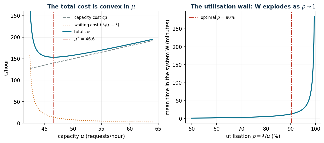
Between \(\rho = 90\%\) and \(\rho = 99\%\) the waiting time is multiplied by ten: "saturating the resources" and "giving good service" are in mathematical, not organizational, conflict.
The price of a service promise
If marketing promises a "mean time below \(w_{\max}\)", we need \(\mu \ge \lambda + 1/w_{\max}\): the constraint becomes active when it is tighter than the economic optimum (13.1 minutes).
w_max = 12 min: mu = 47.00  cost 153.60   (almost free)
w_max =  9 min: mu = 48.67  cost 155.45
w_max =  6 min: mu = 52.00  cost 162.30
w_max =  4 min: mu = 57.00  cost 175.20
w_max =  3 min: mu = 62.00  cost 189.15
w_max =  2 min: mu = 72.00  cost 218.10   (+42% on the base cost)
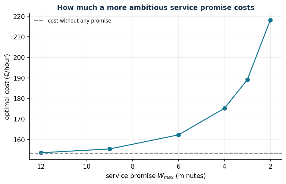
The shadow price of the constraint grows explosively: going from 12 to 9 minutes costs 1.85 €/h, from 3 to 2 minutes costs 28.95 €/h. When the constraint is active, \(\mu = \lambda + 1/w_{\max}\) and \(C = c\lambda + c/w_{\max} + h\lambda\, w_{\max}\), from which \(dC/dw_{\max} = -c/w_{\max}^2 + h\lambda\) (with \(w_{\max}\) in hours): at \(w_{\max} = 6\) minutes it is equal to \(-300 + 63 = -237\) €/h per hour of promise — the number to give to marketing before it signs the SLA (Service Level Agreement).
Robustness: if \(\lambda\) is uncertain in \([36, 48]\), sizing on the nominal optimum \(\tilde\mu = 46{,}58\) is unstable: with \(\lambda = 48 > \tilde\mu\) the queue diverges (infinite cost). Minimizing the cost of the worst case gives \(\mu_{\text{rob}} = 52{,}90\) with a worst-case cost of 173.39 €/h: an insurance premium of about 13% is paid in order to be protected from a disaster.
Code
The complete script of the chapter — data, model, solution, sensitivity and figures —
is python/lab11_queues.py
(reproducible with python3 python/lab11_queues.py from the python/ folder).
The same code is also available as a notebook — notebooks/lab11_queues.ipynb — which opens in Colab from the badge at the top of the page and runs in the browser, with nothing to install.
Show the full script — lab11_queues.py
"""Chapter 11 — Service capacity and waiting times (convex NLP, M/M/1).

Case study: sizing the agents of a customer service desk.
Arrivals lambda = 42 requests/hour; each "capacity unit" mu costs c = 3 €/hour;
one hour spent in the system by a customer is worth h = 1.5 €.

Contents:
  1. Total cost c·mu + h·lambda/(mu-lambda): analytical vs Gurobi (global)
  2. The utilisation wall: rho -> 1 makes the waiting time explode
  3. Service-level constraint W <= W_max and its shadow price
  4. Robustness: lambda uncertain in the interval [36, 48]
"""
import gurobipy as gp
import numpy as np
import pandas as pd
from gurobipy import GRB

from stile import (ARANCIO, GRIGIO, ROSSO, TEAL, VERDE, intestazione, plt, salva_dat,
                   salva_dati, salva_figura)

lam, c, h = 42.0, 3.0, 1.5

# ----------------------------------------------------------------------
# 1. TOTAL COST: analytical vs numerical
# ----------------------------------------------------------------------
intestazione("Analytical and numerical optimum")


def costo(mu):
    return c * mu + h * lam / (mu - lam)


def mu_ottimo(lams):
    """min c·mu + max_l h·l/(mu - l) with Gurobi (global, NonConvex=2).

    The term 1/(mu - l) is linearised with the variable w_l and the bilinear
    constraint w_l·(mu - l) = 1; with a single l this is the basic M/M/1 model,
    with several values of l it is the robust version (worst-case minimisation)."""
    m = gp.Model("mm1")
    m.Params.OutputFlag = 0
    m.Params.NonConvex = 2
    m.Params.MIPGap = 1e-9
    lam_max = max(lams)
    mu = m.addVar(lb=lam_max + 1e-3, ub=4 * lam_max, name="mu")
    t = m.addVar(name="t")                       # t = worst-case waiting cost
    for l in lams:
        w = m.addVar(lb=1e-6, ub=1e5)            # w = 1/(mu - l)
        v = m.addVar(lb=1e-3, ub=4 * lam_max)    # v = mu - l
        m.addConstr(v == mu - l)
        m.addQConstr(w * v == 1)                 # bilinear: solved globally
        m.addConstr(t >= h * l * w)
    m.setObjective(c * mu + t, GRB.MINIMIZE)
    m.optimize()
    assert m.Status == GRB.OPTIMAL
    return mu.X, m.ObjVal


mu_star = lam + np.sqrt(h * lam / c)               # from setting the derivative to zero
mu_num, costo_num = mu_ottimo([lam])
print(f"Analytical: mu* = lambda + sqrt(h·lambda/c) = {mu_star:.3f}  -> cost {costo(mu_star):.3f} €/h")
print(f"Gurobi    : mu* = {mu_num:.3f}  -> cost {costo_num:.3f} €/h")
rho = lam / mu_star
W = 1 / (mu_star - lam)
print(f"At the optimum: utilisation rho = {rho:.1%}, mean time in the system w = {W * 60:.1f} minutes")
print("Note: the optimum is NOT rho ~ 100%: it pays to keep some safety capacity.")

# ----------------------------------------------------------------------
# 2. SERVICE-LEVEL CONSTRAINT: W <= W_max
# ----------------------------------------------------------------------
intestazione("Service level: W <= W_max")
righe = []
for W_max_min in [12, 9, 6, 4, 3, 2]:               # minutes
    W_max = W_max_min / 60
    mu_sl = max(mu_star, lam + 1 / W_max)            # constraint active if more binding
    prezzo_ombra = 0.0
    if mu_sl > mu_star + 1e-9:                       # active constraint: marginal cost
        # dC/dW_max = derivative of the optimal cost with respect to the promise
        eps = 1e-6
        mu_eps = lam + 1 / (W_max + eps)
        prezzo_ombra = (costo(mu_eps) - costo(mu_sl)) / eps
    righe.append((W_max_min, mu_sl, costo(mu_sl), lam / mu_sl, prezzo_ombra))
    print(f"  w_max = {W_max_min:4.1f} min: mu = {mu_sl:7.3f}, cost = {costo(mu_sl):8.3f} €/h, "
          f"rho = {lam / mu_sl:6.1%}, price of the promise = {prezzo_ombra:9.1f} €/h per hour of W")
sl = pd.DataFrame(righe, columns=["W_max_min", "mu", "cost", "rho", "shadow_price"])
salva_dati(sl, "code_service_level")

# ----------------------------------------------------------------------
# 3. ROBUSTNESS: lambda uncertain in [36, 48]
# ----------------------------------------------------------------------
intestazione("Robustness: uncertain demand lambda in [36, 48]")
lam_lo, lam_hi = 36.0, 48.0


mu_rob, costo_rob = mu_ottimo([lam_lo, lam_hi])
print(f"robust mu = {mu_rob:.3f} (vs {mu_star:.3f} nominal)")
print(f"Worst-case cost: {costo_rob:.3f} €/h")
print(f"The nominal plan with lambda = 48 would cost: "
      f"{c * mu_star + h * 48 / (mu_star - 48) if mu_star > 48 else float('inf'):.3f} €/h -> "
      + ("ok" if mu_star > 48 else "UNSTABLE (mu* < maximum lambda!)"))

# ----------------------------------------------------------------------
# 4. FIGURES
# ----------------------------------------------------------------------
mus = np.linspace(lam + 0.4, lam + 22, 400)
salva_dat(pd.DataFrame({"mu": mus, "capacity": c * mus, "waiting": h * lam / (mus - lam),
                        "total": [costo(mm) for mm in mus]}), "cap11_costo")
rhos_ = np.linspace(0.5, 0.995, 300)
salva_dat(pd.DataFrame({"rho": rhos_ * 100, "W_min": 1 / (lam / rhos_ - lam) * 60}),
          "cap11_muro")
salva_dat(sl, "cap11_promessa")
fig, (ax1, ax2) = plt.subplots(1, 2, figsize=(10.5, 4.0))
ax1.plot(mus, c * mus, ls="--", color=GRIGIO, label="capacity cost $c\\mu$")
ax1.plot(mus, h * lam / (mus - lam), ls=":", color=ARANCIO,
         label="waiting cost $h\\lambda/(\\mu-\\lambda)$")
ax1.plot(mus, [costo(mm) for mm in mus], color=TEAL, lw=2, label="total cost")
ax1.axvline(mu_star, color=ROSSO, ls="-.", label=f"$\\mu^*$ = {mu_star:.1f}")
ax1.set_xlabel("capacity $\\mu$ (requests/hour)")
ax1.set_ylabel("€/hour")
ax1.set_ylim(0, 260)
ax1.set_title("The total cost is convex in $\\mu$")
ax1.legend(fontsize=8)

rhos = np.linspace(0.5, 0.995, 300)
ax2.plot(rhos * 100, 1 / (lam / rhos - lam) * 60, color=TEAL, lw=2)
ax2.axvline(rho * 100, color=ROSSO, ls="-.", label=f"optimal $\\rho$ = {rho:.0%}")
ax2.set_xlabel("utilisation $\\rho = \\lambda/\\mu$ (%)")
ax2.set_ylabel("mean time in the system W (minutes)")
ax2.set_title("The utilisation wall: W explodes as $\\rho \\to 1$")
ax2.legend(fontsize=8)
salva_figura(fig, "cap11_costo_muro")

fig, ax = plt.subplots()
ax.plot(sl["W_max_min"], sl["cost"], "-o", color=TEAL)
ax.axhline(costo(mu_star), color=GRIGIO, ls="--", label="cost without any promise")
ax.set_xlabel("service promise $W_{max}$ (minutes)")
ax.set_ylabel("optimal cost (€/hour)")
ax.set_title("How much a more ambitious service promise costs")
ax.invert_xaxis()
ax.legend(fontsize=8)
salva_figura(fig, "cap11_promessa")

print("\nDone: chapter 11.")
Exercises
- Derive \(dC/dw_{\max} = -c/w_{\max}^2 + h\lambda\) and verify it at 4 and 9 minutes.
- Quadratic waiting cost \(h/(\mu - \lambda)^2\): \(\tilde\mu = \lambda + (2h/c)^{1/3}\).
- Pooling: two separate queues (\(\lambda = 21\) each) vs a single one (\(\lambda = 42\)) at equal total capacity.
- Frontier (cost, \(w\)): where does every promised minute cut cost more than 10 €/h? (Below ~4 minutes.)