Continuous location of a service
Lecture notes (PDF) · Chapter slides (PDF)
Class: convex NLP · Script: python/lab09_location.py

Where should a charging station, a micro-hub, a health-care post be placed in order to be "close" to demand? It depends on what close means: mean distance (efficiency), maximum (equity) or squared (centroid). Three objectives, three different points on the map.
The problem in words. We decide the coordinates \((x, y)\). The objective is the real managerial choice (mean / maximum / squared). The constraints delimit the feasible area.
Model
Data (input of the model).
| Symbol | Type | Meaning |
|---|---|---|
| \(n\) | \(\in \mathbb{Z}_{\ge 1}\) | number of demand points (districts), indexed by \(i \in \{1, 2, \dots, n\}\) |
| \((a_i, b_i)\) | \(\in \mathbb{Q}^2\) | coordinates of district \(i\) (km) |
| \(w_i\) | \(\in \mathbb{Q}_{\ge 0}\) | weight of district \(i\): population, demand or priority |
| \((a_0, b_0)\), \(r\) | \(\in \mathbb{Q}^2\), \(\in \mathbb{Q}_{>0}\) | centre and radius of the possible geographic constraint (maximum distance from an infrastructure) |
Decision variables. We introduce the following \(2\) free variables (they may take any real value) and, for the minimax version, a non-negative auxiliary variable:
Using these variables, the models for the three classical objectives are the following. Weber model (weighted mean distance):
Minimax model (maximum distance):
Description of the objective functions and of the constraints of the two models:
- the convex objective function of the Weber model minimizes the total distance weighted by the districts (efficiency); the constraints on \(x\) and \(y\) define the variables, which are free;
- the objective function of the minimax model minimizes the distance of the farthest district (equity); the convex covering constraints impose that every district is at most at distance \(z\) from the facility (\(n\) constraints); the constraints on \(x\), \(y\) and \(z\) define the variables;
- a third variant, quadratic: minimize \(\sum_{i=1}^{n} w_i \bigl[ (x - a_i)^2 + (y - b_i)^2 \bigr]\), which has a closed-form solution (the weighted centroid \(\tilde x = \sum_{i=1}^{n} w_i\, a_i \big/ \sum_{i=1}^{n} w_i\), and analogously for \(y\)).
Typical convex geographic constraints, to be added to any variant: rectangular zone \(x^{L} \le x \le x^{U}\), \(y^{L} \le y \le y^{U}\); maximum distance from an infrastructure \((x - a_0)^2 + (y - b_0)^2 \le r^2\).
The Weber model has no closed form and its objective function is not differentiable at the points \((a_i, b_i)\): at the optimum the weighted unit "pulls" of the districts cancel out. The optimum of the minimax is instead the centre of the smallest enclosing circle of all the points: it depends only on the extreme districts and ignores the weights — this is why it protects the outskirts.
Worked example by hand (1D)
Customers at km 0, 4, 10 with weights 1, 1, 3. Weber = weighted median = 10; centroid = 6.8; minimax = 5. Three reasonable objectives, three different answers: the choice of the objective is the managerial decision.
Case study
12 districts (weights 5–25 thousand inhabitants), constraint: within 2 km of the
electrical substation at (7, 6). Data in data/localizzazione_quartieri.csv.
The modelling trick: a variable \(d_k \ge\) the Euclidean distance from district \(k\), imposed with the (convex) conic constraint \(d_x^2 + d_y^2 \le d_k^2\); Weber minimizes \(\sum_k w_k d_k\), the minimax a variable \(z\) with \(d_k \le z\).
Weighted centroid : (4.897, 5.397)
Weber             : (4.886, 5.310)  mean dist. 3.344 km  max 6.314 km
Minimax           : (5.496, 5.029)  mean dist. 3.391 km  max 5.680 km
Constrained Weber : (5.083, 5.429)  cost +0.2% (constraint active, optimum on boundary)
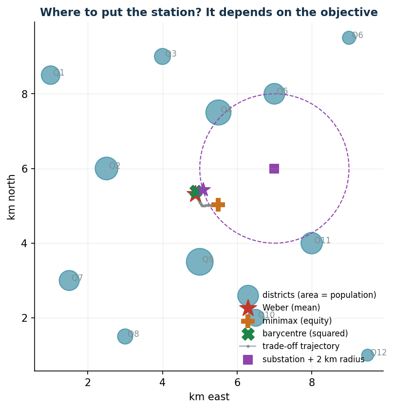
Weber and the centroid almost coincide (the weights are evenly distributed), but the minimax moves more than half a kilometre towards the south-east to protect the peripheral districts; the constraint of the substation costs very little (+0.2%): discovering that a feared constraint is almost free is a managerial result as important as the optimum itself.
Sensitivity: the efficiency-equity frontier
The ε-constraint method: minimum mean distance with a cap \(D\) on the maximum.
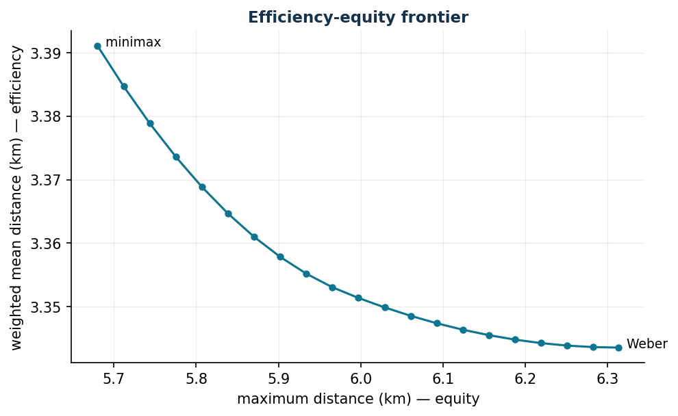
cap D = 5.680 km: mean 3.391   (minimax solution)
cap D = 5.997 km: mean 3.351
cap D = 6.314 km: mean 3.344   (Weber solution)
The frontier is almost flat: guaranteeing 0.63 km less to the farthest district costs only 47 metres of mean distance — equity here is "almost free", a very strong argument in a public discussion. The opposite case (a steep frontier) would signal a genuine efficiency-equity conflict.
Code
The complete script of the chapter — data, model, solution, sensitivity and figures —
is python/lab09_location.py
(reproducible with python3 python/lab09_location.py from the python/ folder).
The same code is also available as a notebook — notebooks/lab09_location.ipynb — which opens in Colab from the badge at the top of the page and runs in the browser, with nothing to install.
Show the full script — lab09_location.py
"""Chapter 9 — Continuous location of a service (convex NLP).

Case study: where to place a fast-charging station in a city with 12 districts,
weighted by population.

Contents:
  1. Weighted barycentre (squared distance): closed-form solution
  2. Weber point (Euclidean distance): Gurobi (conic reformulation)
  3. Minimax (protects the farthest district): reformulation with a variable z
  4. Trade-off alpha·mean + (1-alpha)·maximum: efficiency-equity curve
"""
import gurobipy as gp
import numpy as np
import pandas as pd
from gurobipy import GRB

from stile import (ARANCIO, GRIGIO, ROSSO, TEAL, VERDE, intestazione, plt, salva_dat,
                   salva_dati, salva_figura, salva_tikz)

rng = np.random.default_rng(7)

# ----------------------------------------------------------------------
# 1. DATA: 12 districts (coordinates in km, weight = population in thousands)
# ----------------------------------------------------------------------
nomi = [f"Q{k}" for k in range(1, 13)]
coord = np.array([
    [1.0, 8.5], [2.5, 6.0], [4.0, 9.0], [5.5, 7.5], [7.0, 8.0], [9.0, 9.5],
    [1.5, 3.0], [3.0, 1.5], [5.0, 3.5], [6.5, 2.0], [8.0, 4.0], [9.5, 1.0]])
peso = np.array([12.0, 18.0, 9.0, 22.0, 15.0, 6.0, 14.0, 8.0, 25.0, 10.0, 16.0, 5.0])
salva_dati(pd.DataFrame({"district": nomi, "x": coord[:, 0], "y": coord[:, 1], "weight": peso}),
           "localizzazione_quartieri")


def dist(p):
    return np.sqrt(((coord - p) ** 2).sum(axis=1))


def f_weber(p):
    return float(peso @ dist(p))


def f_max(p):
    return float(dist(p).max())


def localizza(pesi=None, tetto=None, cabina=None, raggio=None):
    """Location with Gurobi (convex SOCP, certified global optimum).

    The trick: a variable d_k >= Euclidean distance from district k, imposed
    with the conic constraint dx_k^2 + dy_k^2 <= d_k^2 (d_k >= 0). With weights
    it minimises the weighted mean distance (Weber); without weights it minimises
    the maximum one (minimax). `tetto` imposes d_k <= cap; `cabina`/`raggio` the
    geographical constraint."""
    m = gp.Model("location")
    m.Params.OutputFlag = 0
    px = m.addVar(lb=-GRB.INFINITY, name="px")
    py = m.addVar(lb=-GRB.INFINITY, name="py")
    n = len(coord)
    d = m.addVars(n, name="d")
    for k in range(n):
        dx = m.addVar(lb=-GRB.INFINITY)
        dy = m.addVar(lb=-GRB.INFINITY)
        m.addConstr(dx == px - coord[k, 0])
        m.addConstr(dy == py - coord[k, 1])
        m.addQConstr(dx * dx + dy * dy <= d[k] * d[k])   # cone: d_k >= distance
    if tetto is not None:
        m.addConstrs((d[k] <= tetto for k in range(n)))
    if cabina is not None:
        m.addQConstr((px - cabina[0]) ** 2 + (py - cabina[1]) ** 2 <= raggio ** 2)
    if pesi is not None:                     # Weber: weighted mean
        m.setObjective(gp.quicksum(pesi[k] * d[k] for k in range(n)), GRB.MINIMIZE)
    else:                                    # minimax: maximum distance
        z = m.addVar(name="z")
        m.addConstrs((d[k] <= z for k in range(n)))
        m.setObjective(z, GRB.MINIMIZE)
    m.optimize()
    assert m.Status == GRB.OPTIMAL
    return np.array([px.X, py.X]), m.ObjVal


# ----------------------------------------------------------------------
# 2. THREE CLASSIC OBJECTIVES
# ----------------------------------------------------------------------
intestazione("Three optimal locations")
baricentro = (peso[:, None] * coord).sum(axis=0) / peso.sum()   # closed form
print(f"Weighted barycentre (squared dist.) : ({baricentro[0]:.3f}, {baricentro[1]:.3f}) km")

weber, costo_weber = localizza(pesi=peso)
print(f"Weber point (weighted mean dist.)   : ({weber[0]:.3f}, {weber[1]:.3f}) km, "
      f"cost {costo_weber:,.1f} (thousand inh. · km)")

minimax, dist_minimax = localizza()
print(f"Minimax (farthest district)         : ({minimax[0]:.3f}, {minimax[1]:.3f}) km, "
      f"maximum distance {dist_minimax:.3f} km")

print(f"\nWith the Weber point: weighted mean distance {f_weber(weber) / peso.sum():.3f} km, "
      f"maximum {f_max(weber):.3f} km")
print(f"With the minimax    : weighted mean distance {f_weber(minimax) / peso.sum():.3f} km, "
      f"maximum {f_max(minimax):.3f} km")

# ----------------------------------------------------------------------
# 3. EFFICIENCY-EQUITY FRONTIER (constraint method, epsilon-constraint):
#    minimise the weighted mean distance imposing max_dist <= D
# ----------------------------------------------------------------------
intestazione("Efficiency-equity frontier (min mean with a cap on the maximum)")
media_pesi = peso.sum()
D_grid = np.linspace(f_max(minimax) + 1e-4, f_max(weber), 21)
punti = []
for D in D_grid:
    pos, _ = localizza(pesi=peso, tetto=D)
    punti.append((D, pos[0], pos[1], f_weber(pos) / media_pesi, f_max(pos)))
comp = pd.DataFrame(punti, columns=["D_max", "x", "y", "mean_dist", "max_dist"])
salva_dati(comp, "localizzazione_frontiera")
for _, r in comp.iloc[::5].iterrows():
    print(f"  cap D = {r['D_max']:5.3f} km: position ({r['x']:5.2f}, {r['y']:5.2f}), "
          f"mean {r['mean_dist']:5.3f} km, max {r['max_dist']:5.3f} km")

# ----------------------------------------------------------------------
# 4. GEOGRAPHICAL CONSTRAINT: within 2 km of an electrical substation
# ----------------------------------------------------------------------
intestazione("Weber with a constraint: within R = 2 km of the substation at (7, 6)")
cabina, R = np.array([7.0, 6.0]), 2.0
pos_v, costo_v = localizza(pesi=peso, cabina=cabina, raggio=R)
print(f"Constrained optimum: ({pos_v[0]:.3f}, {pos_v[1]:.3f}), cost {costo_v:,.1f}")
print(f"Cost of the constraint: +{costo_v - costo_weber:,.1f} with respect to the free Weber "
      f"({(costo_v / costo_weber - 1) * 100:.1f}%)")
attivo = np.isclose(((pos_v - cabina) ** 2).sum(), R**2, rtol=1e-3)
print(f"The constraint is {'active (optimum on the boundary of the circle)' if attivo else 'not active'}")

# ----------------------------------------------------------------------
# 5. FIGURES (generated TikZ + pgfplots data + matplotlib preview)
# ----------------------------------------------------------------------
salva_dat(comp, "cap09_frontiera")

r = ["% Map of the districts and optimal locations (generated by lab09_location.py)",
     "\\begin{tikzpicture}[scale=0.82, >=stealth]",
     "  \\draw[black!20, very thin] (0,0) grid[step=1] (10.5,10);",
     "  \\draw[->, black!50] (0,0) -- (10.8,0) node[below left, font=\\scriptsize] {km east};",
     "  \\draw[->, black!50] (0,0) -- (0,10.3) node[below left, rotate=90, font=\\scriptsize] {km north};"]
for k, nome in enumerate(nomi):
    raggio = 0.11 * np.sqrt(peso[k])
    r.append(f"  \\fill[teal, opacity=0.45] ({coord[k, 0]:.2f},{coord[k, 1]:.2f}) "
             f"circle ({raggio:.2f});")
    r.append(f"  \\node[font=\\tiny, text=black!55, anchor=west] at "
             f"({coord[k, 0] + raggio:.2f},{coord[k, 1]:.2f}) {{{nome}}};")
r.append("  % trajectory of the efficiency-equity trade-off")
traj = " -- ".join(f"({rr['x']:.3f},{rr['y']:.3f})" for _, rr in comp.iterrows())
r.append(f"  \\draw[black!45, thick, densely dotted] {traj};")
r.append(f"  % geographical constraint: circle of the substation")
r.append(f"  \\draw[viola, dashed, thick] ({cabina[0]},{cabina[1]}) circle ({R});")
r.append(f"  \\node[rectangle, fill=viola, minimum size=2.2mm, inner sep=0] at "
         f"({cabina[0]},{cabina[1]}) {{}};")
# labels at different angles to avoid overlaps (the points are close to each other)
punti_not = [(weber, "rossomattone", 190, "Weber"),
             (minimax, "arancio", -55, "minimax"),
             (baricentro, "verde", 120, "barycentre"),
             (pos_v, "viola", 35, "constrained Weber")]
for pt, colore, angolo, etich in punti_not:
    r.append(f"  \\node[star, star points=5, fill={colore}, minimum size=3.2mm, inner sep=0pt,"
             f" label={{[font=\\scriptsize, text={colore}, label distance=2.5mm]"
             f"{angolo}:{etich}}}] at ({pt[0]:.3f},{pt[1]:.3f}) {{}};")
r.append("\\end{tikzpicture}")
salva_tikz("\n".join(r), "cap09_mappa")

fig, ax = plt.subplots(figsize=(7.2, 6.2))
ax.scatter(coord[:, 0], coord[:, 1], s=peso * 28, color=TEAL, alpha=0.55,
           label="districts (area = population)")
for k, nome in enumerate(nomi):
    ax.annotate(f" {nome}", coord[k], fontsize=8, color=GRIGIO)
ax.scatter(*weber, marker="*", s=300, color=ROSSO, zorder=5, label="Weber (mean)")
ax.scatter(*minimax, marker="P", s=160, color=ARANCIO, zorder=5, label="minimax (equity)")
ax.scatter(*baricentro, marker="X", s=140, color=VERDE, zorder=5, label="barycentre (squared)")
ax.plot(comp["x"], comp["y"], ".-", color=GRIGIO, lw=1, ms=4, alpha=0.8,
        label="trade-off trajectory")
cerchio = plt.Circle(cabina, R, fill=False, color="#8E44AD", ls="--")
ax.add_patch(cerchio)
ax.scatter(*cabina, marker="s", s=70, color="#8E44AD", label="substation + 2 km radius")
ax.scatter(*pos_v, marker="*", s=200, color="#8E44AD", zorder=5)
ax.set_xlabel("km east"); ax.set_ylabel("km north")
ax.set_title("Where to put the station? It depends on the objective")
ax.legend(fontsize=8, loc="lower right")
ax.set_aspect("equal")
salva_figura(fig, "cap09_mappa")

fig, ax = plt.subplots()
ax.plot(comp["max_dist"], comp["mean_dist"], "-o", color=TEAL, ms=4)
for idx, etich in [(0, "minimax"), (20, "Weber")]:
    r = comp.iloc[idx]
    ax.annotate(f"  {etich}", (r["max_dist"], r["mean_dist"]), fontsize=9)
ax.set_xlabel("maximum distance (km) — equity")
ax.set_ylabel("weighted mean distance (km) — efficiency")
ax.set_title("Efficiency-equity frontier")
salva_figura(fig, "cap09_frontiera")

print("\nDone: chapter 9.")
Exercises
- Recompute by hand the weighted centroid from the CSV data.
- Weight of Q12 from 5 to 40: Weber migrates by 1.23 km; the minimax does not move (it ignores the weights).
- Two facilities with assignment to the nearest one: why is the problem no longer convex?
- Manhattan distance: show that Weber becomes an LP (weighted medians per coordinate).
- Multiplier of the radius: with \(r = 2 \to 2.1\) the cost drops from 535.79 to 535.22.