Supply chain with congestion and sustainability
Lecture notes (PDF) · Chapter slides (PDF)
Class: LP / convex NLP · Script: python/lab05_supplychain.py

Products cross a network of plants, hubs and markets. Every leg has a cost, a capacity and a CO₂ footprint. How should the flows be routed at minimum cost? What changes if we penalize congestion? How much must CO₂ be worth for the "clean" routes to become convenient?
The problem in words. We decide how many units travel on each leg. The objective: minimum transport cost. The constraints: flow conservation at every node and capacity of the legs.
Model
Data (input of the model).
| Symbol | Type | Meaning |
|---|---|---|
| \(G = (N, A)\) | directed graph | nodes \(N\) and arcs \(A \subseteq N \times N\); we write \(\lvert N \rvert\) and \(\lvert A \rvert\) for the number of nodes and of arcs |
| \(b_i\) | \(\in \mathbb{Q}\) | balance of node \(i \in N\): supply if \(> 0\), demand if \(< 0\), transit if \(= 0\) |
| \(u_{ij}\) | \(\in \mathbb{Q}_{> 0}\) | capacity of arc \((i,j) \in A\) (units) |
| \(c_{ij}\) | \(\in \mathbb{Q}_{\ge 0}\) | transport cost of one unit on arc \((i,j)\) (€) |
| \(e_{ij}\) | \(\in \mathbb{Q}_{\ge 0}\) | emissions per unit transported on \((i,j)\) (kg CO₂) |
Decision variables. We introduce one non-negative variable for each of the \(|A|\) arcs:
Using these variables, an LP model for the problem is the following:
Description of the objective function and of the constraints:
- the linear objective function minimizes the total transport cost: every unit that crosses arc \((i,j)\) pays the unit cost \(c_{ij}\);
- the linear flow conservation constraints impose that at every node what goes out minus what comes in equals the balance \(b_i\) — positive at the plants, negative at the markets, zero at the hubs (\(|N|\) linear constraints); the sum of the balances over all the nodes must be \(\ge 0\), otherwise the model is infeasible;
- the linear capacity constraints ensure that no leg carries more than its own capacity (\(|A|\) linear constraints);
- the non-negativity constraints on \(x_{ij}\) define the variables of the model.
Variants on the objective (the constraints do not change):
where \(\alpha \in \mathbb{Q}_{\ge 0}\) weighs congestion and \(\tau \in \mathbb{Q}_{\ge 0}\) (€/kg) is the internal price of CO₂.
Worked example by hand (two routes)
100 units; route 1: \(c_1 = 2\), \(u_1 = 80\); route 2: \(c_2 = 5\). The LP fills the cheap route (\(x = (80, 20)\), cost 260 €). With congestion (\(\alpha = 1\)) the marginal costs are equalized: \(2 + x_1/20 = 5 \Rightarrow x = (60, 40)\) — the cheap route is no longer saturated.
Case study
2 plants → 2 hubs → 4 markets, 12 arcs; the cheap legs are "by road"
(polluting), the expensive ones "by rail" (clean). Data in data/supplychain_archi.csv.
LP minimum cost : cost 3.385.00 EUR  emissions 2.730 kg  max utilization 100%
  saturated arcs: S1->H1, S2->H2, H2->M3
  shadow prices of demand: M1 8.00  M2 9.50  M3 10.00  M4 10.50 EUR/unit
  reduced costs of arcs at zero (threshold = SAObjLow):
    S2->H1 +2.00 (threshold 5.00)   H1->M4 +0.50 (threshold 5.50)
    H2->M1 +4.50 (threshold 1.50)   H2->M2 +1.00 (threshold 3.00)  EUR/unit
Congestion a=1  : cost 3.702.81 EUR  emissions 2.530 kg  max utilization  90%
Minimax         : minimum possible maximum utilization 58.4%
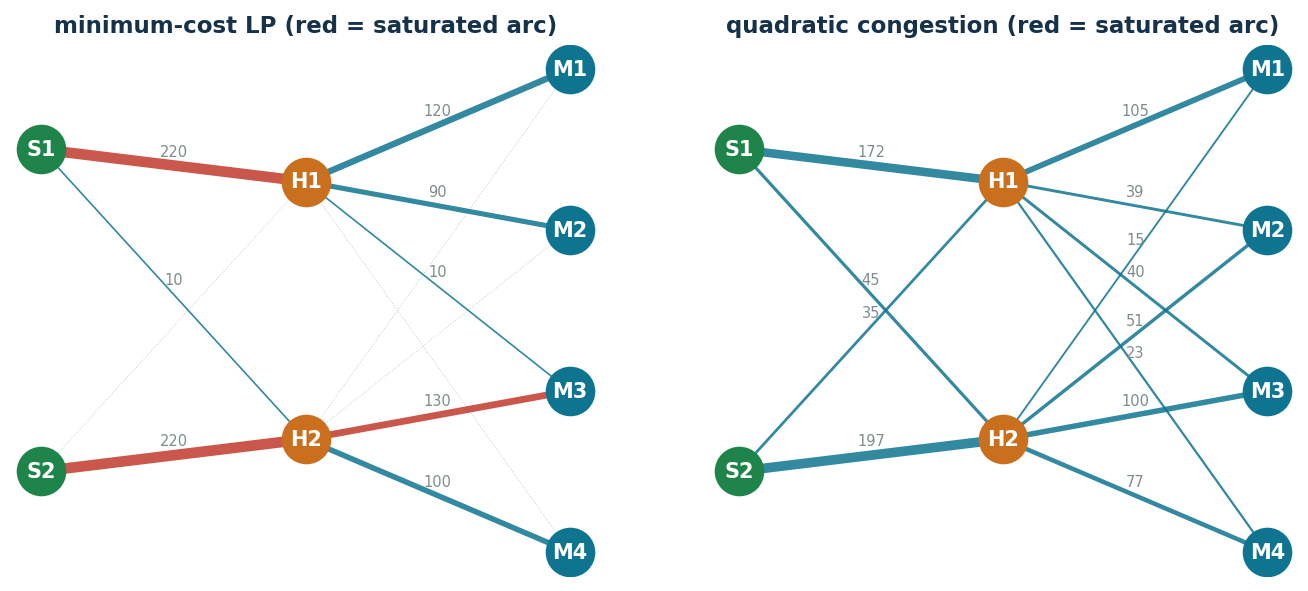
The shadow prices of demand are the marginal costs of service of the markets: the basis for accepting orders and for internal transfer prices.
The reduced costs of the unused arcs (x[a].RC) are their convenience
thresholds: S2→H1 (cost 7 €, RC +2) would enter the solution only below
7 − 2 = 5 €/unit — the number to bring to a negotiation with the carrier; H1→M4 is
one step away from being used (RC +0.50). As always we also quote the range of validity
SAObjLow/Up: for a variable at zero it is \([\text{threshold}, +\infty)\) and the threshold is
exactly SAObjLow. The positive variables have zero reduced cost.
Sensitivity: the price of CO₂
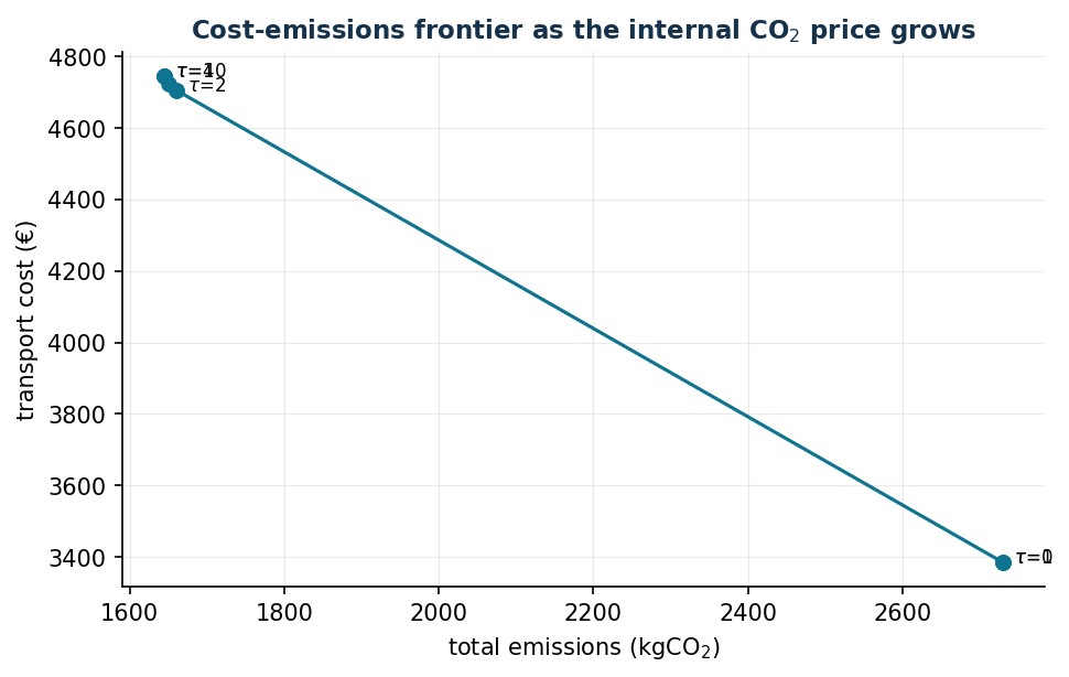
tau = 0.0 ... 1.0 : cost 3385  emissions 2730   (routes by road)
tau = 1.24        : cost 4025  emissions 2173   (intermediate vertex)
tau = 1.26        : cost 4265  emissions 1981
tau = 1.5         : cost 4705  emissions 1661   ("rail" configuration)
tau = 4.0 and up  : cost 4745  emissions 1645   (stable)
The solutions of LPs lie at the vertices: as \(\tau\) grows the optimum stays put on one vertex, then it jumps to the next one. Up to \(\tau = 1\) nothing changes, between \(\tau = 1.0\) and \(\tau = 1.5\) the network crosses intermediate vertices (at \(\tau = 1.24\): 2173 kg) and the main jump happens exactly at \(\tau = 1.25\) €/kg: below the threshold the internal price of CO₂ does not change the routes, just above it, it restructures the whole network at once. The model with congestion, being strictly convex, would instead move continuously.
Degenerate minimax
The "pure" minimax (\(\min z\)) accepts any routing with utilization \(\le \tilde z\), even an extremely expensive one: always combine it with the cost.
Code
The complete script of the chapter — data, model, solution, sensitivity and figures —
is python/lab05_supplychain.py
(reproducible with python3 python/lab05_supplychain.py from the python/ folder).
The same code is also available as a notebook — notebooks/lab05_supplychain.ipynb — which opens in Colab from the badge at the top of the page and runs in the browser, with nothing to install.
Show the full script — lab05_supplychain.py
"""Chapter 5 — Supply chain with congestion and sustainability (LP / convex NLP).

Network: 2 plants (S1, S2) -> 2 hubs (H1, H2) -> 4 markets (M1..M4).

Contents:
  1. Minimum-cost flow (LP) and shadow prices of the saturated arcs
  2. Quadratic congestion: flows spread out to avoid saturation
  3. Internal CO2 price (tau): cost-emissions frontier
  4. Minimax: minimise the maximum utilisation of the network
"""
import gurobipy as gp
import numpy as np
import pandas as pd
from gurobipy import GRB

from stile import (ARANCIO, GRIGIO, ROSSO, TEAL, VERDE, intestazione, plt, salva_dat,
                   salva_dati, salva_figura, salva_tikz)

# ----------------------------------------------------------------------
# 1. DATA
# ----------------------------------------------------------------------
offerta = {"S1": 260, "S2": 240}                     # production capacity (units)
domanda = {"M1": 120, "M2": 90, "M3": 140, "M4": 100}  # demand (units); tot 450 < 500

#           arc: (capacity U, unit cost c €/u, emissions e kgCO2/u)
# emissions are NOT proportional to costs: cheap but polluting arcs (road)
# and expensive but clean arcs (rail) — so the CO2 price shifts the routes
archi = {
    ("S1", "H1"): (220, 4.0, 3.5),
    ("S1", "H2"): (180, 6.5, 1.2),
    ("S2", "H1"): (150, 7.0, 1.5),
    ("S2", "H2"): (220, 3.5, 4.0),
    ("H1", "M1"): (130, 3.0, 2.8),
    ("H1", "M2"): (100, 4.5, 1.0),
    ("H1", "M3"): (120, 5.0, 1.2),
    ("H1", "M4"): (90, 6.0, 1.0),
    ("H2", "M1"): (80, 6.0, 1.1),
    ("H2", "M2"): (90, 4.0, 2.5),
    ("H2", "M3"): (130, 3.5, 3.0),
    ("H2", "M4"): (110, 4.0, 2.4),
}
A = list(archi)
U = {a: archi[a][0] for a in A}
c = {a: archi[a][1] for a in A}
e = {a: archi[a][2] for a in A}
hub = ["H1", "H2"]

salva_dati(pd.DataFrame([(i, j, *archi[i, j]) for (i, j) in A],
                        columns=["from", "to", "capacity", "cost", "emissions"]),
           "supplychain_archi")


def costruisci(tau=0.0, congestione=0.0):
    """Flow model. tau = CO2 price (€/kg); congestione = weight alpha of the
    quadratic term c_ij*x + alpha*c_ij*x^2/U (convex)."""
    m = gp.Model("supply_chain")
    m.Params.OutputFlag = 0
    x = m.addVars(A, name="x", ub=U)
    v_off = m.addConstrs((x.sum(s, "*") <= offerta[s] for s in offerta), name="supply")
    m.addConstrs((x.sum("*", h) == x.sum(h, "*") for h in hub), name="transit")
    v_dom = m.addConstrs((x.sum("*", k) == domanda[k] for k in domanda), name="demand")
    obj = gp.quicksum((c[a] + tau * e[a]) * x[a] for a in A)
    if congestione > 0:
        obj += gp.quicksum(congestione * c[a] * x[a] * x[a] / U[a] for a in A)
    m.setObjective(obj, GRB.MINIMIZE)
    return m, x, v_off, v_dom


def riassunto(x):
    costo = sum(c[a] * x[a].X for a in A)
    co2 = sum(e[a] * x[a].X for a in A)
    util_max = max(x[a].X / U[a] for a in A)
    return costo, co2, util_max


# ----------------------------------------------------------------------
# 2. BASIC LP
# ----------------------------------------------------------------------
intestazione("LP: minimum-cost flow")
m, x, v_off, v_dom = costruisci()
m.optimize()
assert m.Status == GRB.OPTIMAL
costo0, co20, util0 = riassunto(x)
print(f"Transport cost: {costo0:,.2f} €   emissions: {co20:,.1f} kgCO2   "
      f"max arc utilisation: {util0:.0%}")
print("\nOptimal flows (units) and utilisation:")
for a in A:
    if x[a].X > 1e-6:
        print(f"  {a[0]:>2} -> {a[1]:<2}: {x[a].X:6.1f} / {U[a]:3d}  ({x[a].X / U[a]:5.0%})"
              + ("   ** saturated" if x[a].X > U[a] - 1e-6 else ""))
print("\nShadow prices of demand (marginal cost of serving one more unit):")
for k in domanda:
    print(f"  {k}: {v_dom[k].Pi:6.2f} €/unit")
print("\nReduced costs of the unused arcs (how much the unit cost of the arc"
      "\nmust drop for it to enter the optimal solution):")
for a in A:
    if x[a].X < 1e-6:
        print(f"  {a[0]:>2} -> {a[1]:<2}: cost {c[a]:4.1f} €, RC = {x[a].RC:+5.2f} €, "
              f"validity range SAObj = [{x[a].SAObjLow:4.1f}, +inf) "
              f"-> worthwhile below {x[a].SAObjLow:4.1f} €/unit")
salva_dati(pd.DataFrame([(a[0], a[1], x[a].X, x[a].X / U[a]) for a in A],
                        columns=["from", "to", "flow", "utilisation"]), "supplychain_flussi_lp")

# ----------------------------------------------------------------------
# 3. QUADRATIC CONGESTION
# ----------------------------------------------------------------------
intestazione("Quadratic congestion (alpha = 1)")
mc, xc, _, _ = costruisci(congestione=1.0)
mc.optimize()
costoc, co2c, utilc = riassunto(xc)
print(f"Transport cost: {costoc:,.2f} €   emissions: {co2c:,.1f} kgCO2   "
      f"max arc utilisation: {utilc:.0%}")
print("The quadratic term spreads the flows: fewer saturated arcs, higher linear cost.")

# ----------------------------------------------------------------------
# 4. CO2 PRICE: cost-emissions frontier
# ----------------------------------------------------------------------
intestazione("Cost-emissions frontier as the CO2 price varies")
taus = [0, 0.5, 1, 1.5, 2, 3, 4, 6, 8, 10]
frontiera = []
for tau in taus:
    mt, xt, _, _ = costruisci(tau=tau)
    mt.optimize()
    ct, et, ut = riassunto(xt)
    frontiera.append((tau, ct, et))
    print(f"  tau = {tau:4.1f} €/kg: transport cost {ct:8.2f} €, emissions {et:7.1f} kg")
front = pd.DataFrame(frontiera, columns=["tau", "cost", "emissions"])
salva_dati(front, "supplychain_frontiera_co2")

# ----------------------------------------------------------------------
# 5. MINIMAX: minimum maximum utilisation
# ----------------------------------------------------------------------
intestazione("Minimax: minimum maximum utilisation of the network")
mm, xm, _, _ = costruisci()
z = mm.addVar(name="z")
mm.addConstrs((xm[a] / U[a] <= z for a in A), name="load")
mm.setObjective(z, GRB.MINIMIZE)
mm.optimize()
print(f"Lowest achievable maximum utilisation: {mm.ObjVal:.1%} "
      f"(minimum-cost LP: {util0:.0%}, congestion: {utilc:.0%})")

# ----------------------------------------------------------------------
# 6. FIGURES (generated TikZ + pgfplots data + matplotlib preview)
# ----------------------------------------------------------------------
pos = {"S1": (0, 1), "S2": (0, -1), "H1": (1, 0.8), "H2": (1, -0.8),
       "M1": (2, 1.5), "M2": (2, 0.5), "M3": (2, -0.5), "M4": (2, -1.5)}

salva_dat(front, "cap05_frontiera_co2")


def tikz_rete(xx, titolo):
    """Generate the TikZ code of the network with the flows of solution xx."""
    sx, sy = 3.4, 1.15                              # horizontal and vertical scale
    r = []
    r.append(f"% Network of the solution: {titolo} (generated by lab05_supplychain.py)")
    r.append("\\begin{tikzpicture}[>=stealth,")
    r.append("    nodo/.style={circle, draw=none, text=white, font=\\bfseries\\small,")
    r.append("                 minimum size=8mm, inner sep=0pt}]")
    for a in A:
        (x1, y1), (x2, y2) = pos[a[0]], pos[a[1]]
        f = xx[a].X
        if f > 1e-6:
            saturo = f > U[a] - 1e-6
            colore = "rossomattone" if saturo else "teal"
            spess = 0.4 + 1.6 * f / max(U.values())
            r.append(f"  \\draw[{colore}, line width={spess:.2f}pt] "
                     f"({x1 * sx:.2f},{y1 * sy:.2f}) -- ({x2 * sx:.2f},{y2 * sy:.2f})")
            r.append(f"    node[midway, above, sloped, font=\\tiny, text=black!60] "
                     f"{{{f:.0f}}};")
        else:
            r.append(f"  \\draw[black!25, densely dotted, line width=0.4pt] "
                     f"({x1 * sx:.2f},{y1 * sy:.2f}) -- ({x2 * sx:.2f},{y2 * sy:.2f});")
    stile_nodo = {"S": "verde", "H": "arancio", "M": "teal"}
    for nn, (px, py) in pos.items():
        r.append(f"  \\node[nodo, fill={stile_nodo[nn[0]]}] at ({px * sx:.2f},{py * sy:.2f}) "
                 f"{{{nn}}};")
    r.append(f"  \\node[font=\\small\\bfseries, text=blunotte] at ({sx:.2f},{2.0 * sy:.2f}) "
             f"{{{titolo}}};")
    r.append("\\end{tikzpicture}")
    return "\n".join(r)


salva_tikz(tikz_rete(x, "Minimum-cost LP"), "cap05_rete_lp")
salva_tikz(tikz_rete(xc, "Quadratic congestion"), "cap05_rete_congestione")

fig, assi = plt.subplots(1, 2, figsize=(11, 4.6))
for ax, (xx, titolo) in zip(assi, [(x, "minimum-cost LP"), (xc, "quadratic congestion")]):
    for a in A:
        (x1, y1), (x2, y2) = pos[a[0]], pos[a[1]]
        f = xx[a].X
        if f > 1e-6:
            colore = ROSSO if f > U[a] - 1e-6 else TEAL
            ax.plot([x1, x2], [y1, y2], color=colore, lw=0.6 + 4.5 * f / max(U.values()),
                    alpha=0.85, zorder=1)
            ax.annotate(f"{f:.0f}", ((x1 + x2) / 2, (y1 + y2) / 2 + 0.06),
                        fontsize=7, color=GRIGIO, ha="center")
        else:
            ax.plot([x1, x2], [y1, y2], color=GRIGIO, lw=0.5, ls=":", alpha=0.4, zorder=0)
    for n, (px, py) in pos.items():
        col = VERDE if n.startswith("S") else (ARANCIO if n.startswith("H") else TEAL)
        ax.scatter([px], [py], s=520, color=col, zorder=2)
        ax.annotate(n, (px, py), color="white", weight="bold", ha="center", va="center", zorder=3)
    ax.set_title(titolo + " (red = saturated arc)")
    ax.axis("off")
salva_figura(fig, "cap05_reti")

fig, ax = plt.subplots()
ax.plot(front["emissions"], front["cost"], "-o", color=TEAL)
for _, r in front.iterrows():
    if r["tau"] in (0, 1, 2, 4, 10):
        ax.annotate(f"  $\\tau$={r['tau']:.0f}", (r["emissions"], r["cost"]), fontsize=8)
ax.set_xlabel("total emissions (kgCO$_2$)")
ax.set_ylabel("transport cost (€)")
ax.set_title("Cost-emissions frontier as the internal CO$_2$ price grows")
salva_figura(fig, "cap05_frontiera_co2")

print("\nDone: chapter 5.")
Exercises
- Verify by perturbation the shadow prices of M4 and of arc H2→M3 (the latter is saturated but degenerate: zero dual).
- Hub H2 at 50%: how much does the failure cost? (+542.50 €) Which markets suffer?
- Reproduce the threshold \(\tau = 1.25\) and identify the arcs that change.
- Constraint \(\sum e_{ij} x_{ij} \le 2000\) kg: verify that the dual coincides with the threshold \(\tau\).
- Barrier \(\alpha x/(u - x)\) instead of the quadratic congestion: compare.