Asymptotic growth

Part 3 · Asymptotic notation and growth · Chapter 10 · Lecture notes, volume 3 (PDF) · Exercises: Asymptotic growth · App: Orders of growth

Introduction

The number of steps executed by an algorithm is a function of a natural number: the size of its input. Two algorithms that solve the same problem are compared by looking at how fast these functions grow when the input grows, and not at their values on a few small inputs. In this chapter we study the functions of a natural variable that appear in the analysis of algorithms and we compare their orders of growth with the asymptotic notations \(o\), \(\bigO\), \(\Theta\), \(\Omega\) and \(\omega\) introduced in chapter 9 «Asymptotic notation».

The plan of the chapter is the following.

• In Section 10.1 we introduce the five families of increasing functions of a natural variable used in the course: logarithmic, power, exponential, factorial and self-power functions.

• In Section 10.2 we recall the four limits that put these families in order (the hierarchy of infinities).

• In Section 10.3 we express the comparison of two orders of growth with the asymptotic notation, through the limit criterion of chapter 9 «Asymptotic notation». We then derive the hierarchy of the orders of growth, a classification of the orders of growth, and the properties of logarithmic, power, polynomial and exponential functions that are used in the analysis of algorithms.

Prerequisites. The functions of a natural variable are the sequences of the course Mathematical Analysis 1 (fabiofurini.github.io/mathematical-analysis-1/, Italian version fabiofurini.github.io/analisi-matematica-1/). Their limits, and the theorems used to compute them, are not explained again in this chapter: we use them, and we refer to the part Limits of sequences of that course, in particular to the chapters Computing limits of sequences (comparison theorem), Euler's number and Hierarchies of infinities and the ratio test.

10.1 Families of increasing functions of a natural variable

A function of a natural variable is defined on a set of natural numbers of the form \(\N_{\ge n_0} = \{n_0, n_0+1, n_0+2, \dots\}\), and in the analysis of algorithms only its behaviour for large values of \(n\) matters. In chapter 9 «Asymptotic notation» we called a function asymptotically positive if \(f(n) > 0\) for all \(n\) from some value onwards: in the course Mathematical Analysis 1 such properties are said to hold eventually. The following definition describes another property of the same kind.

Definition 10.1: asymptotically increasing function

A function of a natural variable \(f: \N_{\ge n_0} \rightarrow \R\) is asymptotically increasing if there exists \(n_1 \in \N_{\ge n_0}\) such that:

\[\begin{equation*} f(n) < f(n+1), \quad \forall n \in \N_{\ge n_1} \tag{10.1} \end{equation*}\]

• The principal families of asymptotically increasing functions of a natural variable are the following ones.

  1. The logarithmic functions of a natural variable:

     \[\begin{equation*} f: \N_{\ge 1} \rightarrow \R,~~~ f:n \mapsto \log_a n \quad \forall a \in \R_{>1} \tag{10.2} \end{equation*}\]

  2. The power functions of a natural variable:

     \[\begin{equation*} f: \N \rightarrow \R,~~~ f:n \mapsto n^{\alpha} \quad \forall \alpha \in \R_{>0} \tag{10.3} \end{equation*}\]

  3. The exponential functions of a natural variable:

     \[\begin{equation*} f: \N \rightarrow \R,~~~ f:n \mapsto b^{n} \quad \forall b \in \R_{>1} \tag{10.4} \end{equation*}\]

  4. The factorial function of a natural variable:

     \[\begin{equation*} f: \N \rightarrow \R,~~~ f:n \mapsto n! \tag{10.5} \end{equation*}\]

  5. The self-power function of a natural variable:

     \[\begin{equation*} f: \N \rightarrow \R,~~~ f:n \mapsto n^n \tag{10.6} \end{equation*}\]

     where, by convention, we set \(0^0 = 1\).

• All these functions are asymptotically positive, and all of them diverge to \(\ip\) as \(n \rr \ip\). The factorial and the self-power functions are not increasing on their whole domain, since \(0! = 1! = 1\) and \(0^0 = 1^1 = 1\), but they are strictly increasing from \(n = 1\) onwards: this is why we speak of asymptotically increasing functions.

• In these notes \(\ln n = \log_e n\) denotes the natural logarithm, where \(e\) is Euler's number.

Example 10.1: increasing functions of a natural variable

The table reports the values of some increasing functions of a natural variable, computed by increasing \(n\) by one order of magnitude at a time, from \(1\) to \(100\) million. The values of \(\ln n\) and the leading factors of \(2^n\) and \(n!\) are rounded to one decimal digit; the values of \(n^2\) and \(n^n\) are exact.

\(n\)	\(\ln n\)	\(n^2\)	\(2^n\)	\(n!\)	\(n^n\)
\(1=10^0\)	\(0\)	\(1\)	\(2\)	\(1\)	\(1\)
\(10=10^1\)	\(\approx 2.3\)	\(10^2\)	\(\approx 1.0 \cdot 10^{3}\)	\(\approx 3.6\cdot 10^{6}\)	\(10^{10}\)
\(100=10^2\)	\(\approx 4.6\)	\(10^4\)	\(\approx 1.3 \cdot 10^{30}\)	\(\approx 9.3\cdot 10^{157}\)	\(10^{200}\)
\(1{,}000=10^3\)	\(\approx 6.9\)	\(10^6\)	\(\approx 1.1 \cdot 10^{301}\)	\(\approx 4.0\cdot 10^{2{,}567}\)	\(10^{3{,}000}\)
\(10{,}000=10^4\)	\(\approx 9.2\)	\(10^8\)	\(\approx 2.0 \cdot 10^{3{,}010}\)	\(\approx 2.8\cdot 10^{35{,}659}\)	\(10^{40{,}000}\)
\(100{,}000=10^5\)	\(\approx 11.5\)	\(10^{10}\)	\(\approx 1.0 \cdot 10^{30{,}103}\)	\(\approx 2.8\cdot 10^{456{,}573}\)	\(10^{500{,}000}\)
\(10^6\)	\(\approx 13.8\)	\(10^{12}\)	\(\approx 9.9 \cdot 10^{301{,}029}\)	\(\approx 8.3\cdot 10^{5{,}565{,}708}\)	\(10^{6{,}000{,}000}\)
\(10^7\)	\(\approx 16.1\)	\(10^{14}\)	\(\approx 9.0 \cdot 10^{3{,}010{,}299}\)	\(\approx 1.2\cdot 10^{65{,}657{,}059}\)	\(10^{70{,}000{,}000}\)
\(10^8\)	\(\approx 18.4\)	\(10^{16}\)	\(\approx 3.7 \cdot 10^{30{,}102{,}999}\)	\(\approx 1.6\cdot 10^{756{,}570{,}556}\)	\(10^{800{,}000{,}000}\)

To appreciate these numbers, recall that the number of atoms in the observable universe is estimated at about \(10^{82}\), and that a personal computer of 2024 executes about \(10 \cdot 10^9 = 10^{10}\) operations per second (\(10\) GFLOPS). An algorithm that executes \(2^n\) operations on an input with \(n = 100\) needs

\[ \frac{2^{100}}{10^{10}} \text{ seconds} \approx 1.3 \cdot 10^{20} \text{ seconds} \approx 4.0 \cdot 10^{12} \text{ years}, \]

while an algorithm that executes \(n^2\) operations needs \(10^{4}/10^{10} = 10^{-6}\) seconds.

• Figure 10.1 shows the first values of the same functions. Since the values grow very fast, the vertical axis is in logarithmic scale: each horizontal line of the grid corresponds to a multiplication by \(100\).

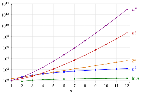
Figure 10.1: The values of \(\ln n\), \(n^2\), \(2^n\), \(n!\) and \(n^n\) for \(n \in \{1, 2, \dots, 12\}\) (vertical axis in logarithmic scale; the points are joined by segments only for readability). For small values of \(n\) the order of the functions can be different from the final one: \(2^3 = 8 < 9 = 3^2\), and \(2^n > n!\) for \(n \in \{1, 2, 3\}\).

10.2 The hierarchy of infinities

The five families of Section 10.1 all diverge to \(\ip\). To decide which one diverges faster, we compute the limit of the ratio of two of them. The limits of this section are the hierarchy of infinities for sequences of the course Mathematical Analysis 1 (chapter Hierarchies of infinities and the ratio test), where they are proved; here we recall them, together with the idea of their proofs, and we extend the first one to the powers of the logarithms.

• Given \(a \in \R_{>1}\) and \(\beta \in \R_{>0}\), the asymptotically increasing function of a natural variable

  \[\begin{equation*} f: \N_{\ge 1} \rightarrow \R,~~~ f:n \mapsto \log^{\beta}_a n = \big(\log_a n\big)^{\beta} \tag{10.7} \end{equation*}\]

  is called a polylogarithmic function of a natural variable.

Proposition 10.2: logarithms and powers

For every \(\alpha \in \R_{>0}\), \(\beta \in \R_{>0}\) and \(a \in \R_{>1}\), we have:

\[\begin{equation*} \lim_{n \rr \ip} \frac{\log_a^\beta n}{n^\alpha} = 0^+ \tag{10.8} \end{equation*}\]

Proof

For \(\beta = 1\) this is the hierarchy of infinities (part I) of the course Mathematical Analysis 1:

\[ \lim_{n \rr \ip} \frac{\log_a n}{n^\alpha} = 0^+, \quad \forall \alpha \in \R_{>0},~ \forall a \in \R_{>1}. \]

It is proved with the inequality \(\log_a x < x \, \log_a 2\), valid for every \(x \in \R_{>0}\) (a consequence of Bernoulli's inequality), applied to \(x = n^{\alpha/2}\), and with the comparison theorem.

For every \(\beta \in \R_{>0}\), since \(\frac{\alpha}{\beta} \in \R_{>0}\), we then have:

\[ \lim_{n \rr \ip} \frac{\log_a^\beta n}{n^\alpha} = \lim_{n \rr \ip} \Bigg( \underbrace{\frac{\log_a n}{n^{\alpha/\beta}}}_{\rr\, 0^+} \Bigg)^{\beta} = 0^+ \]

□

Proposition 10.3: powers and exponentials

For every \(\alpha \in \R_{>0}\) and \(b \in \R_{>1}\), we have:

\[\begin{equation*} \lim_{n \rr \ip} \frac{n^{\alpha}}{b^{n}} = 0^+ \tag{10.9} \end{equation*}\]

• This is the hierarchy of infinities (part II). It follows from Proposition 10.2 by replacing \(n\) with \(2^n\), which gives \(\frac{n}{(2^{\mu})^n} \rr 0^+\) for every \(\mu \in \R_{>0}\), hence \(\frac{n}{b^n} \rr 0^+\) for every \(b \in \R_{>1}\) (choose \(\mu\) such that \(2^{\mu} = b\)); the general case follows from the identity

  \[ \frac{n^\alpha}{b^n} = \left( \frac{n}{\big(b^{1/\alpha}\big)^n} \right)^{\alpha}, \qquad b^{1/\alpha} \in \R_{>1}. \]

Proposition 10.4: exponentials and factorial

For every \(b \in \R_{>1}\), we have:

\[\begin{equation*} \lim_{n \rr \ip} \frac{b^{n}}{n!} = 0^+ \tag{10.10} \end{equation*}\]

• This is the hierarchy of infinities (part III). It follows from the ratio test, since

  \[ \frac{b^{n+1}}{(n+1)!} \; \frac{n!}{b^n} = \frac{b}{n+1} \rr 0^+ < 1. \]

Proposition 10.5: factorial and self-power

\[\begin{equation*} \lim_{n \rr \ip} \frac{n!}{n^n} = 0^+ \tag{10.11} \end{equation*}\]

• This is the hierarchy of infinities (part IV). It follows from the ratio test, since

  \[ \frac{(n+1)!}{(n+1)^{n+1}} \; \frac{n^n}{n!} = \left( \frac{n}{n+1}\right)^n = \frac{1}{\left( 1 + \frac{1}{n} \right)^n} \rr \frac{1}{e} < 1. \]

Polylogarithmic functions (with base greater than one) diverge more slowly than power functions (with positive exponent), which diverge more slowly than exponential functions (with base greater than one), which diverge more slowly than the factorial function, which diverges more slowly than the self-power function.

10.3 Comparison of orders of growth

• The order of growth of an asymptotically increasing function of a natural variable describes how rapidly its values increase compared to the values of another asymptotically increasing function of a natural variable.

• We compare orders of growth with the asymptotic notations \(o\), \(\bigO\), \(\Theta\), \(\Omega\) and \(\omega\) of chapter 9 «Asymptotic notation». For the functions of this chapter the ratio \(\frac{f(n)}{g(n)}\) always has a limit, and the notations that hold are decided by the limit criterion proved there, which we recall.

Proposition 10.6: limit criterion

Let \(f\) and \(g\) be two asymptotically positive functions of a natural variable such that the limit

\[ L = \lim_{n \rr \ip} \frac{f(n)}{g(n)} \]

exists (\(L = 0^+\), \(L \in \R_{>0}\) or \(L = \ip\)). Then:

\[\begin{align*} f(n) = o\big(g(n)\big) &~~\Longleftrightarrow~~ L = 0^+,\\ f(n) = \bigO\big(g(n)\big) &~~\Longleftrightarrow~~ L = 0^+ \ \text{ or } \ L \in \R_{>0},\\ f(n) = \Theta\big(g(n)\big) &~~\Longleftrightarrow~~ L \in \R_{>0},\\ f(n) = \Omega\big(g(n)\big) &~~\Longleftrightarrow~~ L \in \R_{>0} \ \text{ or } \ L = \ip,\\ f(n) = \omega\big(g(n)\big) &~~\Longleftrightarrow~~ L = \ip. \end{align*}\]

• The proof is in chapter 9 «Asymptotic notation» (Proposition «limit criterion»), where the five notations are defined through positive constants and a threshold. In this chapter we compute the limit of the ratio and apply Proposition 10.6.

Given two asymptotically increasing functions of a natural variable \(f\) and \(g\):

• if \(f(n) = o\big(g(n)\big)\), \(f\) has a strictly smaller order of growth than \(g\), \(\rightsquigarrow\) the function \(f\) grows slower than the function \(g\);

• if \(f(n) = \bigO\big(g(n)\big)\), \(f\) has a smaller or equal order of growth compared to \(g\), \(\rightsquigarrow\) the function \(f\) grows at most as fast as the function \(g\);

• if \(f(n) = \Theta\big(g(n)\big)\), \(f\) has the same order of growth as \(g\), \(\rightsquigarrow\) the function \(f\) grows as fast as the function \(g\);

• if \(f(n) = \Omega\big(g(n)\big)\), \(f\) has a greater or equal order of growth compared to \(g\), \(\rightsquigarrow\) the function \(f\) grows at least as fast as the function \(g\);

• if \(f(n) = \omega\big(g(n)\big)\), \(f\) has a strictly greater order of growth than \(g\), \(\rightsquigarrow\) the function \(f\) grows faster than the function \(g\).

• The notations do not depend on the values of \(f\) and \(g\) on finitely many natural numbers: changing them changes neither the limit of the ratio nor, with a larger threshold, the inequalities of the definitions.

• By the relational properties of chapter 9 «Asymptotic notation» (symmetry and transpose symmetry), exchanging the two functions exchanges \(o\) with \(\omega\) and \(\bigO\) with \(\Omega\), while \(\Theta\) does not change:

  \[ f(n) = o\big(g(n)\big) \iff g(n) = \omega\big(f(n)\big), \qquad f(n) = \Theta\big(g(n)\big) \iff g(n) = \Theta\big(f(n)\big). \]

  All five notations are also transitive: for example, \(f(n) = o\big(g(n)\big)\) and \(g(n) = o\big(h(n)\big)\) give \(f(n) = o\big(h(n)\big)\).

Example 10.2: the limit of the ratio

We compare three pairs of functions; the three ratios are drawn in Figure 10.2.

• We have \(\ln n = o\big(\sqrt{n}\big)\), since by Proposition 10.2 (with \(a = e\), \(\beta = 1\), \(\alpha = \frac{1}{2}\)):

  \[ \lim_{n \rr \ip} \frac{\ln n}{\sqrt n} = 0^+ \]

• We have \(2n^2 + 3n = \Theta(n^2)\), since:

  \[ \lim_{n \rr \ip} \frac{2n^2+3n}{n^2} = \lim_{n \rr \ip} \Big( 2 + \underbrace{\frac{3}{n}}_{\rr\, 0} \Big) = 2 \in \R_{>0} \]

• We have \(n \ln n = \omega(n)\), since:

  \[ \lim_{n \rr \ip} \frac{n \ln n}{n} = \lim_{n \rr \ip} \ln n = \ip \]

The first ratio is not monotone: it increases up to its largest value, about \(0.74\), reached for \(n = 7\), and only then it decreases towards \(0\).

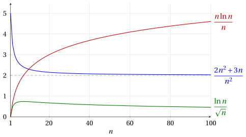
Figure 10.2: The three ratios of [Example 10.2](#box-9-gr-exRatios) for \(n \in \{1, 2, \dots, 100\}\) (the points are joined by segments). The first one tends to \(0\), the second one to \(2\) (dashed line), the third one diverges to \(\ip\).

• Proposition 10.6 requires the limit of the ratio to exist. For example, for \(f(n) = n\) if \(n\) is even and \(f(n) = 2n\) if \(n\) is odd, the ratio \(\frac{f(n)}{n}\) takes alternately the values \(1\) and \(2\) and has no limit; nevertheless \(f(n) = \Theta(n)\), by the definition of chapter 9 «Asymptotic notation» with \(c_1 = 1\), \(c_2 = 2\) and \(n_1 = 0\), since \(0 \le n \le f(n) \le 2n\) for every \(n \in \N\). All the comparisons of this chapter are made between functions whose ratio has a limit.

10.3.1 Hierarchy of the orders of growth

By Proposition 10.6, the limits of Section 10.2 translate directly into relations \(o\) between the families.

• Any polylogarithmic function of a natural variable with a base strictly greater than one is \(o\) of any power function of a natural variable with a positive exponent.

Observation 10.7: polylogarithms and powers

For every \(\alpha \in \R_{>0}\), \(\beta \in \R_{>0}\) and \(a \in \R_{>1}\), we have \(\log^{\beta}_a n = o(n^{\alpha})\).

Proof

By Proposition 10.2, for every \(\alpha \in \R_{>0}\), \(\beta \in \R_{>0}\) and \(a \in \R_{>1}\), we have:

\[ \lim_{n \rr \ip} \frac{\log^{\beta}_a n}{n^{\alpha}} = 0^+ \]

and the claim follows from Proposition 10.6. □

• Any power function of a natural variable with a positive exponent is \(o\) of any exponential function of a natural variable with a base strictly greater than one.

Observation 10.8: powers and exponentials

For every \(\alpha \in \R_{>0}\) and \(b \in \R_{>1}\), we have \(n^{\alpha} = o(b^{n})\).

Proof

By Proposition 10.3, for every \(\alpha \in \R_{>0}\) and \(b \in \R_{>1}\), we have:

\[ \lim_{n \rr \ip} \frac{n^{\alpha}}{b^{n}} = 0^+ \]

and the claim follows from Proposition 10.6. □

Example 10.3: comparison of orders of growth

• We have \(\ln^6 n + 2 + 2^{1/n} + 3^{-n} + 9\,n^2 = o(n^3)\), since:

  \[ \lim_{n \rr \ip} \frac{\ln^6 n + 2 + 2^{1/n} + 3^{-n} + 9\,n^2}{n^3} = \lim_{n \rr \ip} \Bigg( \underbrace{\frac{\ln^6 n}{n^3}}_{\rr\, 0^+} + \underbrace{\frac{2}{n^3}}_{\rr\, 0^+} + \underbrace{\frac{2^{1/n}}{n^3}}_{\rr\, 0^+} + \underbrace{\frac{3^{-n}}{n^3}}_{\rr\, 0^+} + \underbrace{\frac{9}{n}}_{\rr\, 0^+} \Bigg) = 0^+ \]

• We have \(3n^2 + \sqrt{n} + \ln n + 5 + 4^{-n} + 10\,n^{1/3} = o(n^3)\), since:

  \[ \lim_{n \rr \ip} \frac{3n^2 + \sqrt{n} + \ln n + 5 + 4^{-n} + 10\,n^{1/3}}{n^3} = \lim_{n \rr \ip} \Bigg( \underbrace{\frac{3}{n}}_{\rr\, 0^+} + \underbrace{\frac{1}{n^{5/2}}}_{\rr\, 0^+} + \underbrace{\frac{\ln n}{n^3}}_{\rr\, 0^+} + \underbrace{\frac{5}{n^3}}_{\rr\, 0^+} + \underbrace{\frac{4^{-n}}{n^3}}_{\rr\, 0^+} + \underbrace{\frac{10}{n^{8/3}}}_{\rr\, 0^+} \Bigg) = 0^+ \]

• We have \(n^{1/4} + \ln^2 n + \frac{7}{\sqrt{n}} + e^{-n} + 20\,n^{1/2} = o(n^2)\), since:

  \[ \lim_{n \rr \ip} \frac{n^{1/4} + \ln^2 n + \frac{7}{\sqrt{n}} + e^{-n} + 20\,n^{1/2}}{n^2} = \lim_{n \rr \ip} \Bigg( \underbrace{\frac{1}{n^{7/4}}}_{\rr\, 0^+} + \underbrace{\frac{\ln^2 n}{n^2}}_{\rr\, 0^+} + \underbrace{\frac{7}{n^{5/2}}}_{\rr\, 0^+} + \underbrace{\frac{e^{-n}}{n^2}}_{\rr\, 0^+} + \underbrace{\frac{20}{n^{3/2}}}_{\rr\, 0^+} \Bigg) = 0^+ \]

In each case the terms with a logarithm go to \(0^+\) by Proposition 10.2, the other terms by elementary limits, and the claim follows from Proposition 10.6.

• Any exponential function of a natural variable with a base strictly greater than one is \(o\) of the factorial function of a natural variable.

Observation 10.9: exponentials and factorial

For every \(b \in \R_{>1}\), we have \(b^{n} = o(n!)\).

Proof

By Proposition 10.4, for every \(b \in \R_{>1}\), we have:

\[ \lim_{n \rr \ip} \frac{b^{n}}{n!} = 0^+ \]

and the claim follows from Proposition 10.6. □

• The factorial function of a natural variable is \(o\) of the self-power function of a natural variable.

Observation 10.10: factorial and self-power

We have \(n! = o(n^n)\).

Proof

By Proposition 10.5, we have:

\[ \lim_{n \rr \ip} \frac{n!}{n^n} = 0^+ \]

and the claim follows from Proposition 10.6. □

Example 10.4: comparison with the self-power function

We have \(n! + 2^n + \sqrt{n} + \ln^3 n + n^{n-1} + \frac{1}{n} = o(n^n)\), since:

\[ \lim_{n \rr \ip} \frac{n! + 2^n + \sqrt{n} + \ln^3 n + n^{n-1} + \frac{1}{n}}{n^{n}} = \lim_{n \rr \ip} \Bigg( \underbrace{\frac{n!}{n^{n}}}_{\rr\, 0^+} + \underbrace{\frac{2^n}{n^{n}}}_{\rr\, 0^+} + \underbrace{\frac{\sqrt{n}}{n^{n}}}_{\rr\, 0^+} + \underbrace{\frac{\ln^3 n}{n^{n}}}_{\rr\, 0^+} + \underbrace{\frac{1}{n}}_{\rr\, 0^+} + \underbrace{\frac{1}{n^{n+1}}}_{\rr\, 0^+} \Bigg) = 0^+ \]

For example, \(\frac{2^n}{n^n} = \frac{2^n}{n!} \, \frac{n!}{n^n}\) is the product of two functions that tend to \(0^+\), by Propositions 10.4 and Proposition 10.5.

Hierarchy of the orders of growth. For every \(a \in \R_{>1}\), \(\beta \in \R_{>0}\), \(\alpha \in \R_{>0}\) and \(b \in \R_{>1}\), we have

\[ \log_a^\beta n = o(n^\alpha), \qquad n^\alpha = o(b^n), \qquad b^n = o(n!), \qquad n! = o(n^n). \]

By the transitivity of \(o\) (chapter 9 «Asymptotic notation»), each function of the chain is \(o\) of all the functions that follow it, for example \(\log_a^\beta n = o(n!)\).

10.3.2 Classification of orders of growth

The families of the hierarchy are used as yardsticks to classify the order of growth of any other function.

Definition 10.11: bounded orders of growth

An asymptotically increasing function of a natural variable \(f\) has:

• a polylogarithmically bounded order of growth, if there exists \(\beta \in \R_{>0}\) such that \(f(n) = \bigO(\ln^{\beta} n)\); and a logarithmically bounded order of growth, if \(f(n) = \bigO(\ln n)\);

• a polynomially bounded order of growth, if there exists \(\alpha \in \R_{>0}\) such that \(f(n) = \bigO(n^{\alpha})\);

• an exponentially bounded order of growth, if there exists \(b \in \R_{>1}\) such that \(f(n) = \bigO(b^{n})\);

• a factorially bounded order of growth, if \(f(n) = \bigO(n!)\).

Definition 10.12: linear, sub-linear and super-linear order of growth

An asymptotically increasing function of a natural variable \(f\) has:

• a sub-linear order of growth, if \(f(n) = o(n)\);

• a linear order of growth, if \(f(n) = \Theta(n)\);

• a super-linear order of growth, if \(f(n) = \omega(n)\).

• By the hierarchy of the orders of growth, a function with a polylogarithmically bounded order of growth has also a polynomially bounded order of growth, which in turn is also exponentially bounded and factorially bounded. For example, \(f(n) = \bigO(\ln^{\beta} n)\) and \(\ln^{\beta} n = o(n)\) give \(f(n) = \bigO(n)\), since \(o\) implies \(\bigO\) and \(\bigO\) is transitive (chapter 9 «Asymptotic notation»).

Example 10.5: classification of orders of growth

We classify four functions, drawn in Figure 10.3.

• \(\sqrt n = o(n)\), since \(\frac{\sqrt n}{n} = \frac{1}{\sqrt n} \rr 0^+\): a sub-linear order of growth. It has a polynomially bounded order of growth, since \(\sqrt n = \bigO(n^{1/2})\), but not a polylogarithmically bounded one: since \(\frac{\ln^{\beta} n}{\sqrt n} \rr 0^+\) (Proposition 10.2), we have \(\frac{\sqrt n}{\ln^{\beta} n} \rr \ip\), that is, \(\sqrt n = \omega(\ln^{\beta} n)\) and \(\sqrt n \neq \bigO(\ln^{\beta} n)\) for every \(\beta \in \R_{>0}\) (Proposition 10.6).

• \(n = \Theta(n)\): a linear order of growth.

• \(n \ln n = \omega(n)\), since \(\frac{n \ln n}{n} = \ln n \rr \ip\): a super-linear order of growth. It has a polynomially bounded order of growth, since \(\frac{n \ln n}{n^2} = \frac{\ln n}{n} \rr 0^+\), so that \(n \ln n = o(n^2)\) and \(n \ln n = \bigO(n^2)\).

• \(n^2 = \omega(n)\), since \(\frac{n^2}{n} = n \rr \ip\): a super-linear order of growth. It has a polynomially bounded order of growth, since \(n^2 = \bigO(n^2)\).

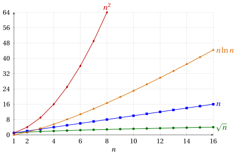
Figure 10.3: A sub-linear function (\(\sqrt n\)), the linear function \(n\) and two super-linear functions (\(n \ln n\) and \(n^2\)) for \(n \in \{1, 2, \dots, 16\}\) (\(n^2\) only up to \(n = 8\), where it reaches \(64\); the points are joined by segments).

10.3.3 Properties of logarithmic functions

In the proofs of this subsection and of the following ones we compute the limit of the ratio of the two functions and we apply Proposition 10.6.

• Any two logarithmic functions of a natural variable with bases strictly greater than one are \(\Theta\) of each other; multiplying the argument by a positive constant does not change the order of growth either.

Observation 10.13: change of base

For every \(a \in \R_{>1}\), \(c \in \R_{>1}\) and \(\lambda \in \R_{>0}\), we have \(\log_{a} (\lambda\, n) = \Theta(\log_{c} n)\).

Proof

For every \(a,c \in \R_{>1}\) and \(\lambda \in \R_{>0}\), since \(\log_a (\lambda\, n) = \log_a \lambda + \log_a n\) and \(\log_a n = \frac{\log_c n}{\log_c a}\), we have:

\[ \lim_{n \rr \ip} \frac{\log_{a}(\lambda\, n)}{\log_c n} = \lim_{n \rr \ip} \Bigg( \underbrace{\frac{\log_a \lambda}{\log_c n}}_{\rr\, 0} + \frac{\frac{\log_c n}{\log_c a}}{\log_c n} \Bigg) = \frac{1}{\log_c a} \in \R_{>0} \]

□

• For this reason, when only the order of growth matters, the base of a logarithm is often omitted. For example, \(\log_2 n = \Theta(\ln n)\), and \(\lim_{n \rr \ip} \frac{\log_2 n}{\ln n} = \frac{1}{\ln 2} \approx 1.44\).

• Adding a positive constant to the argument of a logarithmic function of a natural variable does not change its order of growth.

Observation 10.14: shift of the argument

For every \(a \in \R_{>1}\) and \(\lambda \in \R_{>0}\), we have \(\log_{a} (n+\lambda) = \Theta(\log_{a} n)\).

Proof

For every \(a \in \R_{>1}\) and \(\lambda \in \R_{>0}\), we have:

\[ \lim_{n \rr \ip} \frac{\log_a (n+\lambda)}{\log_a n} = \lim_{n \rr \ip} \frac{\log_a \left(n \left(1 + \frac{\lambda}{n} \right)\right)}{\log_a n} = \lim_{n \rr \ip} \frac{\log_a n + \overbrace{\log_a \left(1+\frac{\lambda}{n}\right)}^{\rr\, 0}}{\log_a n} = 1 \]

□

• The quasi-linear function of a natural variable \(n \mapsto n \log_a n\) is \(o\) of any power function of a natural variable with exponent strictly greater than one.

Observation 10.15: quasi-linear and powers

For every \(\alpha \in \R_{>1}\) and \(a \in \R_{>1}\), we have \(n \log_a n = o(n^{\alpha})\).

Proof

For every \(\alpha \in \R_{>1}\) and \(a \in \R_{>1}\), we have \(\alpha - 1 \in \R_{>0}\) and, by Proposition 10.2:

\[ \lim_{n \rr \ip} \frac{n \log_a n}{n^{\alpha}} = \lim_{n \rr \ip} \frac{\log_a n}{n^{\alpha-1}} = 0^+ \]

□

• The quasi-linear function of a natural variable \(n \mapsto n \log_a n\) is \(\omega\) of the linear function of a natural variable: it has a super-linear order of growth.

Observation 10.16: quasi-linear and linear

For every \(a \in \R_{>1}\), we have \(n \log_a n = \omega(n)\).

Proof

For every \(a \in \R_{>1}\), we have:

\[ \lim_{n \rr \ip} \frac{n \log_a n}{n} = \lim_{n \rr \ip} \log_a n = \ip \]

□

10.3.4 Properties of power functions

• Adding a positive constant to the argument of a power function of a natural variable does not change its order of growth.

Observation 10.17: shift of the argument

For every \(\alpha \in \R_{>0}\) and \(\lambda \in \R_{>0}\), we have \((n+\lambda)^{\alpha} = \Theta(n^{\alpha})\).

Proof

For every \(\alpha \in \R_{>0}\) and \(\lambda \in \R_{>0}\), we have:

\[ \lim_{n \rr \ip} \frac{(n+\lambda)^{\alpha}}{n^{\alpha}} = \lim_{n \rr \ip} \Big(1 + \underbrace{\frac{\lambda}{n}}_{\rr\, 0} \Big)^{\alpha} = 1 \]

□

• Multiplying the argument of a power function of a natural variable by a positive constant does not change its order of growth.

Observation 10.18: scaling of the argument

For every \(\alpha \in \R_{>0}\) and \(\lambda \in \R_{>0}\), we have \((\lambda\, n)^{\alpha} = \Theta(n^{\alpha})\).

Proof

For every \(\alpha \in \R_{>0}\) and \(\lambda \in \R_{>0}\), we have:

\[ \lim_{n \rr \ip} \frac{(\lambda\, n)^{\alpha}}{n^{\alpha}} = \lim_{n \rr \ip} \frac{\lambda^{\alpha}\, n^{\alpha}}{n^{\alpha}} = \lambda^{\alpha} \in \R_{>0} \]

□

• The order of growth of a power function of a natural variable, compared to the linear function of a natural variable, depends on whether the exponent is greater or smaller than one.

Observation 10.19: powers and the linear function

For every \(\alpha \in \R_{>0}\), we have:

• \(n^{\alpha} = \omega(n)\) (super-linear order of growth), if \(\alpha > 1\);

• \(n^{\alpha} = o(n)\) (sub-linear order of growth), if \(\alpha < 1\).

Proof

For every \(\alpha \in \R_{>0}\), we have:

\[ \lim_{n \rr \ip} \frac{n^{\alpha}}{n} = \lim_{n \rr \ip} n^{\alpha - 1} = \begin{cases} \ip & \text{if} ~~~ \alpha > 1\\[1ex] 0^+ & \text{if} ~~~ \alpha < 1 \end{cases} \]

□

10.3.5 Properties of polynomial functions

• Any polynomial function of a natural variable of degree \(k\) with a positive leading coefficient is \(\Theta(n^k)\): it has the same order of growth as its leading term.

Observation 10.20: polynomials

For every \(k \in \N_{\ge 1}\) and every \(a_0, a_1, \dots, a_k \in \R\) with \(a_k \in \R_{>0}\), we have \(\sum_{i=0}^{k} a_i \, n^i = \Theta(n^k)\).

Proof

We have:

\[ \lim_{n \rr \ip} \frac{\sum_{i=0}^{k} a_i \, n^i}{n^{k}} = a_k + \lim_{n \rr \ip} \sum_{i=0}^{k-1} \underbrace{\frac{a_i}{n^{k-i}}}_{\rr\, 0} = a_k \in \R_{>0} \]

In particular, the polynomial is asymptotically positive, so Proposition 10.6 applies. □

10.3.6 Properties of exponential functions

• Any exponential function of a natural variable with a base strictly greater than one is \(\omega\) of the exponential functions of a natural variable with a smaller base, and \(o\) of the exponential functions of a natural variable with a greater base.

Observation 10.21: different bases

For every \(b \in \R_{>1}\) and \(c \in \R_{>1}\), we have:

• \(b^n = \omega(c^n)\), if \(b > c\);

• \(b^n = o(c^n)\), if \(b < c\).

Proof

For every \(b \in \R_{>1}\) and \(c \in \R_{>1}\), since \(b = c^{\log_c b}\), we have:

\[ \lim_{n \rr \ip} \frac{b^n}{c^n} = \lim_{n \rr \ip} \frac{c^{n \log_c b}}{c^n} = \lim_{n \rr \ip} \Big(c^{\log_c b-1}\Big)^{n} = \begin{cases} \ip & \text{if} ~~~ b > c\\[1ex] 0^+ & \text{if} ~~~ b < c \end{cases} \]

since \(c^{\log_c b - 1} = \frac{b}{c}\) is greater than one if \(b > c\) and belongs to \((0,1)\) if \(b < c\) (limit of the geometric progression). □

• Multiplying the exponent of an exponential function of a natural variable by a positive constant changes its order of growth, unless the constant is equal to one.

Observation 10.22: scaling of the exponent

For every \(b \in \R_{>1}\) and \(\lambda \in \R_{>0}\), we have:

• \(b^{\lambda n} = \omega(b^n)\), if \(\lambda > 1\);

• \(b^{\lambda n} = o(b^n)\), if \(0 < \lambda < 1\).

Proof

For every \(b \in \R_{>1}\) and \(\lambda \in \R_{>0}\), we have:

\[ \lim_{n \rr \ip} \frac{b^{\lambda n}}{b^n} = \lim_{n \rr \ip} \left(\frac{b^{\lambda}}{b}\right)^n = \lim_{n \rr \ip} \left(b^{\lambda-1}\right)^n = \begin{cases} \ip & \text{if} ~~~ \lambda > 1\\[1ex] 0^+ & \text{if} ~~~ 0 < \lambda < 1 \end{cases} \]

□

• An alternative proof is based on the fact that

  \[ b^{\lambda n} = \big( b^{\lambda} \big)^n \qquad \text{and} \qquad b^{\lambda} \begin{cases} > b & \text{if} ~~~ \lambda > 1\\[1ex] < b & \text{if} ~~~ 0 < \lambda < 1 \end{cases} \]

  Accordingly, by Observation 10.21 applied to the bases \(b^{\lambda}\) and \(b\), we have \(b^{\lambda n} = \omega(b^n)\) if \(\lambda > 1\), and \(b^{\lambda n} = o(b^n)\) if \(0 < \lambda < 1\).

Example 10.6: scaling the exponent

• We have \(2^{n/2} = o(2^n)\), since

  \[ 2^{n/2} = \big(2^{1/2}\big)^{n} \qquad \text{and} \qquad 2^{1/2} = \sqrt 2 < 2. \]

• We have \(2^{3n/2} = \omega(2^n)\), since

  \[ 2^{3n/2} = \big(2^{3/2}\big)^{n} \qquad \text{and} \qquad 2^{3/2} = 2\sqrt 2 > 2. \]

• Shifting the exponent of an exponential function of a natural variable by a constant does not change its order of growth.

Observation 10.23: shift of the exponent

For every \(b \in \R_{>1}\) and \(\lambda \in \R\), we have \(b^{n+\lambda} = \Theta(b^{n})\).

Proof

For every \(b \in \R_{>1}\) and \(\lambda \in \R\), we have:

\[ \lim_{n \rr \ip} \frac{b^{n+\lambda}}{b^n} = \lim_{n \rr \ip} \frac{b^{n}\, b^{\lambda}}{b^n} = b^{\lambda} \in \R_{>0} \]

□

• For example, \(2^{n+10} = 1024 \cdot 2^n = \Theta(2^n)\), while \(2^{2n} = 4^n = \omega(2^n)\): a constant added to the exponent is a constant factor, a constant factor in the exponent changes the base.

Key points of the chapter

• The functions of a natural variable used in the analysis of algorithms are logarithmic (\(\log_a n\)), power (\(n^\alpha\)), exponential (\(b^n\)), factorial (\(n!\)) and self-power (\(n^n\)) functions, together with their sums and products.

• The orders of growth are compared with the asymptotic notation of chapter 9 «Asymptotic notation». When the limit of \(\frac{f(n)}{g(n)}\) exists it decides (limit criterion): \(0^+\) gives \(f(n) = o\big(g(n)\big)\), a positive real number gives \(f(n) = \Theta\big(g(n)\big)\), \(\ip\) gives \(f(n) = \omega\big(g(n)\big)\).

• Hierarchy (with \(a, b > 1\) and \(\alpha, \beta > 0\)): \(\log_a^\beta n = o(n^\alpha)\), \(n^\alpha = o(b^n)\), \(b^n = o(n!)\), \(n! = o(n^n)\).

• The base of a logarithm, a constant added to the argument of a logarithm or of a power, a constant factor in the argument of a power, and a constant added to the exponent of an exponential do not change the order of growth (the two functions are \(\Theta\) of each other); a polynomial of degree \(k\) with positive leading coefficient is \(\Theta(n^k)\).

• A constant factor in the exponent of an exponential, and a different base of an exponential, do change the order of growth: for example \(2^{n/2} = o(2^n)\) and \(3^n = \omega(2^n)\).

• A function has a sub-linear, linear or super-linear order of growth if it is \(o(n)\), \(\Theta(n)\) or \(\omega(n)\); for example \(\sqrt n\), \(5n+3\) and \(n \ln n\).

---

Exercises on this chapter: Asymptotic growth

Interactive lab

The algorithm of the chapter, one step at a time: move the sliders and press ▶. The same graph full page, with the other ones of the course, is in the interactive lab.