Recursive versus iterative algorithms

Part 5 · Recursion · Chapter 18 · Lecture notes, volume 5 (PDF) · Exercises: Recursive versus iterative algorithms

Introduction

In the previous chapters we have studied several recursive algorithms (chapter «Recursion»: factorial, Fibonacci numbers, recursive GCD, fast power, Tower of Hanoi; chapter «Recursive algorithms»: sum of an array, Merge Sort, Recursive Binary Search, maximum subarray) and we have analysed them by means of recurrences and of the Master Theorem. In this chapter we answer a very practical question:

when is it convenient to design a recursive algorithm, and when is it not?

We will see that the answer does not depend on recursion itself, but on how the problem is decomposed into subproblems:

• if the problem is split into a few independent subproblems of size \(n/b\) (divide and conquer), recursion may give a large asymptotic gain;

• if the problem is only reduced from size \(n\) to size \(n-1\), recursion gives no gain in time and it costs memory;

• if the subproblems overlap, a naive recursive algorithm may be exponentially slower than an iterative one.

The chapter first explains the costs that every recursive call carries, then compares recursive and iterative algorithms for the problems of the course, studies the three situations above one by one, and closes with measured running times of the C++ implementations and with some guidelines.

18.1 Recursion and iteration

Every recursive algorithm can be transformed into an iterative one (that uses an explicit stack to store the pending calls), and every iterative algorithm can be written recursively (every loop can be replaced by a function that calls itself).

Recursion and iteration have the same expressive power: what changes from one to the other is the number of steps and the amount of memory needed to solve the problem.

18.1.1 The hidden costs of recursion

• Each time a function is called, the computer creates a stack frame (or activation record) on the call stack, a memory area reserved to the program. The stack frame contains:

  • the parameters of the call;

  • the local variables of the call;

  • the return address, i.e., the point of the calling function from which the execution resumes when the call terminates.

• The frame is removed from the stack only when the call terminates. Accordingly, during the execution of a recursive algorithm, all the calls that have started and not yet terminated keep their frame on the stack.

• This produces three hidden costs, which do not appear in a loop:

  1. Call overhead: creating and removing a frame, copying the parameters and jumping to the function and back require a constant number of extra steps for each call. This does not change the order of growth of the running time, but it makes a recursive algorithm slower than an equivalent loop by a constant factor.

  2. Memory: the memory used by the call stack is proportional to the maximum number of calls that are simultaneously active, i.e., to the depth of the recursion (the height of the recursion tree plus one, studied in detail later in this chapter).

  3. Stack overflow: the call stack has a fixed and rather small size. On Linux the default size is typically \(8\) MB (command ulimit -s \(\Rightarrow\) \(8192\) KB), on Windows it is typically \(1\) MB. If the depth of the recursion is too large, the stack is exhausted and the program crashes (in C++ with a segmentation fault). In Python the default limit is only \(1000\) nested calls.

Example 18.1: a recursive linear sum that crashes

• Consider the decrease-by-one recursive algorithm that computes the sum of an array \(a[1..n]\) as \(\texttt{SumDecrease}(a,n)=\texttt{SumDecrease}(a,n-1)+a[n]\), with base case \(\texttt{SumDecrease}(a,0)=0\) (the decrease-by-one sum of the chapter «Recursive algorithms», with base case \(n=0\) instead of \(n=1\)).

• The calls \(\texttt{SumDecrease}(a,n), \texttt{SumDecrease}(a,n-1), \dots, \texttt{SumDecrease}(a,0)\) are all active at the same time: the depth of the recursion is \(n+1\).

• With \(n=10^7\) and a stack frame of about \(32\) bytes, the stack should contain about

  \[ 10^7\cdot 32 = 3.2\cdot 10^8 \text{ bytes} \approx 320 \text{ MB}, \]

  i.e., \(40\) times the default \(8\) MB.

• The program crashes, although the array itself (\(4\cdot 10^7\) bytes \(=40\) MB) fits easily in memory and the iterative sum computes the result in about \(3\) milliseconds. In the experiment at the end of the chapter we measure that, with a stack of \(8\) MB, the crash occurs already for \(n\approx 7\cdot 10^5\).

18.1.2 From recursion to iteration with an explicit stack

• A recursive algorithm can always be transformed into an iterative one by managing explicitly a stack that contains the parameters of the calls still to be executed.

• As an example, this is an iterative version of the halving recursive sum RecursiveSum of the chapter «Recursive algorithms», which computes the sum of \(a[l..r]\) as the sum of \(a[l..mid]\) plus the sum of \(a[mid+1..r]\):

Algorithm: SumExplicitStack

Input: An array \(a[1..n]\) of \(n \ge 1\) integer numbers

Output: The sum \(a[1]+a[2]+\cdots+a[n]\)

1function SumExplicitStack(a, n)

2\(s := 0\)

3\(P :=\) empty stack// pending sub-arrays

4push \((1,n)\) on \(P\)

5while \(P\) is not empty do

6\((l,r) :=\) pop from \(P\)

7if \(l = r\) then

8\(s \leftarrow s + a[l]\)// base case

9else

10\(mid := \lfloor (l+r)/2 \rfloor\)

11push \((mid+1,r)\) on \(P\)

12push \((l,mid)\) on \(P\)

13end

14end

15return \(s\)

16end

Run in Colab:PythonC++Java

• The stack \(P\) plays exactly the role of the call stack: it contains the sub-arrays still to be summed. Its maximum size is of the same order as the depth of the recursion, i.e., \(\Theta(\log_2 n)\).

Example 18.2: SumExplicitStack on four elements

We execute SumExplicitStack\((a,4)\) with \(a=[4,7,1,9]\). Each item reports the pair popped from \(P\), what is done, and the content of \(P\) afterwards (the top of the stack is on the right):

• pop \((1,4)\): \(mid=2\), push \((3,4)\) and \((1,2)\) \(\Rightarrow\) \(P=[(3,4),(1,2)]\), \(s=0\);

• pop \((1,2)\): \(mid=1\), push \((2,2)\) and \((1,1)\) \(\Rightarrow\) \(P=[(3,4),(2,2),(1,1)]\), \(s=0\);

• pop \((1,1)\): base case, \(s=4\) \(\Rightarrow\) \(P=[(3,4),(2,2)]\);

• pop \((2,2)\): base case, \(s=11\) \(\Rightarrow\) \(P=[(3,4)]\);

• pop \((3,4)\): \(mid=3\), push \((4,4)\) and \((3,3)\) \(\Rightarrow\) \(P=[(4,4),(3,3)]\), \(s=11\);

• pop \((3,3)\): base case, \(s=12\) \(\Rightarrow\) \(P=[(4,4)]\);

• pop \((4,4)\): base case, \(s=21\) \(\Rightarrow\) \(P\) is empty.

The algorithm returns \(21=4+7+1+9\). The sub-arrays are processed in the same order as the calls of RecursiveSum\((a,1,4)\), and \(P\) never contains more than \(3\) pairs.

Simulating the recursion with an explicit stack does not change the order of growth of the number of steps and of the memory: it only removes the call overhead and moves the stack from the (small) call stack to the (large) main memory.

A real gain in time or in memory can only come from a different algorithm, not from the mechanical replacement of recursion by iteration (or vice versa).

18.2 Comparison at a glance

• The following table compares, for the problems studied in the course, the best iterative algorithm of the course with the recursive one.

• Time is the worst-case number of steps \(S(n)\) (arithmetic operations on numbers are counted as one step, as in the chapter «Running time»); space is the memory used in addition to the input, including the call stack.

• The verdict refers to the recursive algorithm: GAIN if it is asymptotically faster, SAME if it has the same running time, LOSS if it is worse in time or in space.

Problem	Iterative	time	space	Recursive	time	space	Verdict
Sorting	Insertion, Selection, Exchange Sort	\(\Theta(n^2)\)	\(\Theta(1)\)	Merge Sort	\(\Theta(n\log_2 n)\)	\(\Theta(n)\)	GAIN in time (divide and conquer), paid with \(\Theta(n)\) memory
Power \(x^n\)	\(n\) multiplications	\(\Theta(n)\)	\(\Theta(1)\)	Fast power	\(\Theta(\log_2 n)\)	\(\Theta(\log_2 n)\)	GAIN, which comes from halving \(n\): the iterative square-and-multiply is also \(\Theta(\log_2 n)\), with \(\Theta(1)\) space
Maximum subarray	Brute force	\(\Theta(n^2)\)	\(\Theta(1)\)	Divide and conquer	\(\Theta(n\log_2 n)\)	\(\Theta(\log_2 n)\)	GAIN over brute force, but the iterative Kadane algorithm, \(\Theta(n)\) time and \(\Theta(1)\) space, beats both
Product of \(n\)-digit integers	Schoolbook	\(\Theta(n^2)\)	\(\Theta(n)\)	Karatsuba	\(\Theta(n^{\log_2 3})\)	\(\Theta(n)\)	GAIN: \(S(n)=3S(n/2)+\Theta(n)\), \(n^{\log_2 3}\approx n^{1.585}\)
Array sum	Loop	\(\Theta(n)\)	\(\Theta(1)\)	Halving Decr. by one	\(\Theta(n)\) \(\Theta(n)\)	\(\Theta(\log_2 n)\) \(\Theta(n)\)	SAME time, LOSS in space
Binary search	Loop	\(\Theta(\log_2 n)\)	\(\Theta(1)\)	Recursive Binary Search	\(\Theta(\log_2 n)\)	\(\Theta(\log_2 n)\)	SAME time, LOSS in space; tail recursion, it can be removed
Factorial, linear search	Loop	\(\Theta(n)\)	\(\Theta(1)\)	Decrease by one	\(\Theta(n)\)	\(\Theta(n)\)	SAME time, LOSS in space, risk of stack overflow
GCD (Euclid)	Loop	\(\Theta(\log m)\)	\(\Theta(1)\)	Recursive GCD	\(\Theta(\log m)\)	\(\Theta(\log m)\)	SAME: tail recursion, the depth is only logarithmic
Fibonacci numbers	Loop with two variables	\(\Theta(n)\)	\(\Theta(1)\)	Naive recursion	\(\Theta(\varphi^n)\)	\(\Theta(n)\)	huge LOSS: overlapping subproblems; memoization brings it back to \(\Theta(n)\)
Tower of Hanoi	Iterative versions exist	\(\Theta(2^n)\)	\(\Theta(n)\)	Recursive Hanoi	\(\Theta(2^n)\)	\(\Theta(n)\)	SAME: \(2^n-1\) moves are needed anyway; recursion is the natural description

• In the table, \(\varphi=\frac{1+\sqrt5}{2}\approx 1.618\) is the golden ratio and \(m=\min(a,b)\) for the GCD of \(a\) and \(b\).

• The four rows of the first block are the cases where recursion pays off: in all of them the problem is split into subproblems of size \(n/2\) (next section).

• The rows of the second block are the cases where recursion only replaces a loop: no gain in time, a loss in memory (section «Space»).

• The Fibonacci row is the case where naive recursion is a disaster, because the same subproblems are solved over and over again (section «When subproblems overlap»).

18.3 Divide and conquer is what gives the gain, not recursion itself

• The number of steps of a recursive algorithm is described by a recurrence. Two families of recurrences appear in the course:

  • decrease by one: the problem of size \(n\) is reduced to one problem of size \(n-1\),

    \[ S(n)=S(n-1)+f(n); \]

  • divide and conquer: the problem of size \(n\) is split into \(a\) problems of size \(n/b\),

    \[ S(n)=a\,S(n/b)+f(n), \qquad a\ge 1,~b>1. \]

18.3.1 Decrease by one: recursion is a loop in disguise

Observation 18.1: decrease-by-one recurrences

Let \(S(n)=S(n-1)+f(n)\) for \(n\ge 1\), with \(S(0)=d\). Then

\[ S(n)=d+\sum_{i=1}^{n}f(i). \]

In particular, if \(f(n)=c\) for a constant \(c>0\), then \(S(n)=c\,n+d=\Theta(n)\).

Proof

By induction on \(n\). For \(n=0\) the sum is empty and \(S(0)=d\). If the formula holds for \(n-1\), then

\[ S(n)=S(n-1)+f(n)=d+\sum_{i=1}^{n-1}f(i)+f(n)=d+\sum_{i=1}^{n}f(i). \]

If \(f(i)=c\) for every \(i\), then \(\sum_{i=1}^{n}c=c\,n\) and \(S(n)=c\,n+d\). Since \(\lim_{n\to\infty}\frac{c\,n+d}{n}=c\in\R_{>0}\), we have \(S(n)=\Theta(n)\). □

• The formula \(S(n)=d+\sum_{i=1}^{n}f(i)\) is exactly the number of steps of a loop that executes, for \(i=1,2,\dots,n\), a body of cost \(f(i)\). The decrease-by-one recursion does the same work as a loop:

  • factorial, linear search and the decrease-by-one array sum: \(S(n)=S(n-1)+\Theta(1)=\Theta(n)\), like the corresponding loop;

  • a recursive insertion sort (sort \(a[1..n-1]\) recursively, then insert \(a[n]\)): \(S(n)=S(n-1)+\Theta(n)=\Theta(n^2)\), like the iterative InsertionSort.

• In all these cases the recursive algorithm has the same order of growth of the running time as the iterative one, plus the call overhead and a depth of recursion \(\Theta(n)\).

18.3.2 Divide and conquer: where the gain comes from

• Merge Sort splits the array into two halves, sorts them recursively and merges them in \(\Theta(n)\) steps:

  \[ S(n)=2S(n/2)+\Theta(n)=\Theta(n\log_2 n) \]

  by case 2 of the Master Theorem. The gain with respect to \(\Theta(n^2)\) comes from the fact that the two halves are balanced and independent: the recursion tree has only \(\Theta(\log_2 n)\) levels, and each level costs \(\Theta(n)\).

• The same splitting can be organised without recursion: we first merge pairs of sub-arrays of length \(1\), then pairs of sub-arrays of length \(2\), then of length \(4\), and so on. This is the bottom-up Merge Sort. It uses the procedure Merge\((a,l,m,r)\) of the chapter «Recursive algorithms», which merges the sorted sub-arrays \(a[l..m]\) and \(a[m+1..r]\) in \(\Theta(r-l+1)\) steps.

Algorithm: MergeSortBottomUp

Input: An array \(a[1..n]\) of \(n\) natural numbers

Output: The array \(a\) sorted in non-decreasing order

1function MergeSortBottomUp(a, n)

2\(width := 1\)

3while \(width < n\) do

4\(l := 1\)

5while \(l + width \le n\) do

6\(m := l + width - 1\)

7\(r := \min(l + 2\cdot width - 1,~ n)\)

8Merge\((a, l, m, r)\)

9\(l \leftarrow l + 2\cdot width\)

10end

11\(width \leftarrow 2\cdot width\)

12end

13end

Run in Colab:PythonC++Java

Example 18.3: bottom-up Merge Sort

Consider \(a=[5,2,4,6,1,3]\) (\(n=6\)).

• \(width=1\): merge \(a[1..1]\) with \(a[2..2]\), \(a[3..3]\) with \(a[4..4]\), \(a[5..5]\) with \(a[6..6]\) \(\Rightarrow\) \(a=[2,5,4,6,1,3]\).

• \(width=2\): merge \(a[1..2]\) with \(a[3..4]\); for \(l=5\) we have \(l+width=7>6\), so \(a[5..6]\) is left as it is \(\Rightarrow\) \(a=[2,4,5,6,1,3]\).

• \(width=4\): merge \(a[1..4]\) with \(a[5..6]\) \(\Rightarrow\) \(a=[1,2,3,4,5,6]\).

• \(width=8\ge 6\): stop.

The algorithm executes \(3=\lceil \log_2 6\rceil\) passes.

Observation 18.2: bottom-up Merge Sort

For \(n\ge 2\), MergeSortBottomUp executes \(\lceil \log_2 n\rceil\) passes of the outer loop and its number of steps in the worst case is

\[ S(n)=\Theta(n\log_2 n), \]

the same as the recursive Merge Sort. Moreover, it does not use the call stack.

Proof

Let \(n\ge 2\). In the outer loop \(width\) takes the values \(1,2,4,\dots,2^{p-1}\), where \(p\) is the smallest integer with \(2^{p}\ge n\), i.e., \(p=\lceil\log_2 n\rceil\).

Upper bound. In a pass, the calls to Merge (line 8) work on disjoint sub-arrays, so their total length is at most \(n\) and their total cost is \(O(n)\). The inner loop is executed at most \(\frac{n}{2\cdot width}+1\le n\) times, each time with a constant number of other steps. Hence every pass costs \(O(n)\) and \(S(n)=O(n\lceil\log_2 n\rceil)=O(n\log_2 n)\).

Lower bound. The inner loop stops when \(l+width>n\), so the elements that are not merged in a pass are at most \(width\). In the passes with \(width\le n/2\), at least \(n-width\ge n/2\) elements are merged, with \(\Omega(n)\) steps. These passes are those with \(width=2^t\), \(t=0,1,\dots,\lfloor\log_2 n\rfloor-1\), i.e., \(\lfloor\log_2 n\rfloor\) passes. Hence \(S(n)=\Omega(n\lfloor\log_2 n\rfloor)=\Omega(n\log_2 n)\).

Therefore \(S(n)=\Theta(n\log_2 n)\). The algorithm contains no recursive call, so the only extra memory is the one used by Merge, i.e., \(\Theta(n)\). □

The gain of Merge Sort over the \(\Theta(n^2)\) sorting algorithms is a consequence of the divide and conquer strategy (balanced halves, merged in linear time), not of recursion: the iterative bottom-up version has the same running time \(\Theta(n\log_2 n)\).

18.3.3 Fast power: the gain comes from halving

• The recursive fast power of the chapter «Recursion» computes \(x^n=\left(x^{\lfloor n/2\rfloor}\right)^2\) if \(n\) is even, and \(x^n=\left(x^{\lfloor n/2\rfloor}\right)^2\cdot x\) if \(n\) is odd, with \(S(n)=S(\lfloor n/2\rfloor)+\Theta(1)=\Theta(\log_2 n)\).

• Halving the exponent can also be done with a loop, by reading the bits of \(n\) from the least significant one (square-and-multiply):

Algorithm: PowerIt

Input: A number \(x\) and a natural number \(n\)

Output: The power \(x^n\)

1function PowerIt(x, n)

2\(p := 1\)

3\(y := x\)

4\(k := n\)

5while \(k > 0\) do

6if \(k\) is odd then

7\(p \leftarrow p\cdot y\)

8end

9\(y \leftarrow y\cdot y\)

10\(k \leftarrow \lfloor k/2\rfloor\)

11end

12return \(p\)

13end

Run in Colab:PythonC++Java

• At the beginning of each iteration we have \(p\cdot y^{k}=x^n\) (it holds at the start with \(p=1\), \(y=x\), \(k=n\), and it is preserved by every iteration); when \(k=0\) we get \(p=x^n\).

Example 18.4: square-and-multiply with \(n=13\)

We execute PowerIt\((x,13)\), where \(13=(1101)_2\). Each item reports the values at the end of an iteration:

• \(k=13\) is odd: \(p=x\), \(y=x^2\), \(k=6\);

• \(k=6\) is even: \(p=x\), \(y=x^4\), \(k=3\);

• \(k=3\) is odd: \(p=x\cdot x^4=x^5\), \(y=x^8\), \(k=1\);

• \(k=1\) is odd: \(p=x^5\cdot x^8=x^{13}\), \(y=x^{16}\), \(k=0\).

The iterations multiply \(p\) by \(x\), \(x^4\) and \(x^8\) (the bits of \(13\) equal to \(1\)), and \(p=x^{1+4+8}=x^{13}\) after \(4=\lfloor\log_2 13\rfloor+1\) iterations.

Observation 18.3: iterations of PowerIt

For \(n\ge 1\), PowerIt executes exactly \(\lfloor \log_2 n\rfloor+1\) iterations, hence \(S(n)=\Theta(\log_2 n)\), and it uses \(\Theta(1)\) extra memory.

Proof

Every iteration replaces \(k\) by \(\lfloor k/2\rfloor\), i.e., it removes the least significant bit of the binary representation of \(k\). Hence the number of iterations is the number of binary digits of \(n\), which is \(\lfloor\log_2 n\rfloor+1\) (chapter «Representation of numbers»). Each iteration executes a constant number of steps, so \(S(n)=\Theta(\log_2 n)\). Only the three variables \(p\), \(y\), \(k\) are used. □

18.3.4 Maximum subarray: a better iterative algorithm

• For the maximum subarray problem (chapter «Recursive algorithms») the divide and conquer algorithm, with \(S(n)=2S(n/2)+\Theta(n)=\Theta(n\log_2 n)\), improves on the \(\Theta(n^2)\) brute force algorithm.

• However, a smarter iterative algorithm, due to Kadane, solves the problem in \(\Theta(n)\) steps. For each position \(i\) it maintains the maximum sum \(cur\) of a sub-array ending at position \(i\): such a sub-array either is \(a[i]\) alone, or extends the best sub-array ending at \(i-1\). This is a compact version of the algorithm Kadane of the chapter «Recursive algorithms», which returns only the maximum sum:

Algorithm: Kadane

Input: An array \(a[1..n]\) of \(n\ge 1\) integer numbers

Output: The maximum sum of a non-empty sub-array \(a[l..r]\)

1function Kadane(a, n)

2\(best := a[1]\)

3\(cur := a[1]\)// best sum of a sub-array ending at \(i\)

4\(i := 2\)

5while \(i \le n\) do

6\(cur \leftarrow \max(a[i],~ cur + a[i])\)

7\(best \leftarrow \max(best,~ cur)\)

8\(i \leftarrow i+1\)

9end

10return \(best\)

11end

Run in Colab:PythonC++Java

• The loop is executed \(n-1\) times with a constant number of steps: \(S(n)=\Theta(n)\), with \(\Theta(1)\) extra memory.

• Divide and conquer is a powerful design technique, but it is not always the best one: a gain with respect to brute force does not mean that the recursive algorithm is optimal.

18.3.5 Integer multiplication: Karatsuba

• Two \(n\)-digit integers are multiplied with the schoolbook method in \(\Theta(n^2)\) steps on the digits.

• Splitting each number into two halves of \(n/2\) digits, the product requires four products of \(n/2\)-digit numbers. Karatsuba observed that three products are enough (plus additions and shifts, costing \(\Theta(n)\)):

  \[ S(n)=3S(n/2)+\Theta(n). \]

• Here \(a=3\), \(b=2\), \(f(n)=\Theta(n)\) and \(n^{\log_2 3}\approx n^{1.585}\); since \(f(n)=O(n^{\log_2 3-\varepsilon})\) for \(\varepsilon=0.5\), case 1 of the Master Theorem gives \(S(n)=\Theta(n^{\log_2 3})\), asymptotically better than \(\Theta(n^2)\).

Key points. A decrease-by-one recursion does the same work as a loop. A divide and conquer recursion can be asymptotically faster than the simple iterative algorithms (Merge Sort, fast power, Karatsuba), but the gain comes from the decomposition into balanced independent subproblems, and the same decomposition can often be organised with a loop (bottom-up Merge Sort, square-and-multiply). The best algorithm for a problem may even be iterative (Kadane).

18.4 When subproblems overlap

• In divide and conquer the subproblems are disjoint: the two halves of Merge Sort have no element in common. When the subproblems overlap, a naive recursive algorithm solves the same subproblem many times.

• The Fibonacci numbers are defined by \(F(0)=0\), \(F(1)=1\) and \(F(n)=F(n-1)+F(n-2)\) for \(n\ge 2\). The direct translation of the definition is:

Algorithm: FibRec

Input: A natural number \(n\)

Output: The Fibonacci number \(F(n)\)

1function FibRec(n)

2if \(n \le 1\) then

3return \(n\)

4end

5return \(\texttt{FibRec}(n-1) + \texttt{FibRec}(n-2)\)

6end

Run in Colab:PythonC++Java

Example 18.5: the recursion tree of FibRec\((5)\)

This is the recursion tree of \(\texttt{FibRec}(5)\) (each node is a call, labelled with its parameter). The sub-tree of \(\texttt{FibRec}(3)\) is computed twice, the call \(\texttt{FibRec}(2)\) three times:

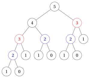
The tree has \(15\) nodes, while only \(6\) different values \(F(0),F(1),\dots,F(5)\) are needed.

Observation 18.4: number of calls of FibRec

For every \(n\ge 0\), the number of calls executed by \(\texttt{FibRec}(n)\) is

\[ C(n)=2F(n+1)-1. \]

Proof

The calls satisfy \(C(0)=C(1)=1\) and \(C(n)=1+C(n-1)+C(n-2)\) for \(n\ge 2\). We prove the formula by strong induction. Base cases: \(C(0)=1=2F(1)-1\) and \(C(1)=1=2F(2)-1\). If the formula holds for \(n-1\) and \(n-2\), then

\[ C(n)=1+\big(2F(n)-1\big)+\big(2F(n-1)-1\big)=2\big(F(n)+F(n-1)\big)-1=2F(n+1)-1. \qedhere \]

□

Observation 18.5: growth of the Fibonacci numbers

Let \(\varphi=\frac{1+\sqrt5}{2}\). For every \(n\ge 1\),

\[ \varphi^{n-2}\le F(n)\le \varphi^{n-1}. \]

Hence \(F(n)=\Theta(\varphi^n)\) and the number of steps of FibRec is \(S(n)=\Theta(C(n))=\Theta(\varphi^n)\).

Proof

The number \(\varphi\) satisfies \(\varphi^2=\varphi+1\). Base cases: \(\varphi^{-1}\approx 0.618\le F(1)=1\le\varphi^0=1\) and \(\varphi^{0}=1\le F(2)=1\le\varphi\approx 1.618\). For \(n\ge 3\), by strong induction,

\[ F(n)=F(n-1)+F(n-2)\ge \varphi^{n-3}+\varphi^{n-4}=\varphi^{n-4}(\varphi+1)=\varphi^{n-4}\varphi^2=\varphi^{n-2}, \]

and in the same way \(F(n)\le\varphi^{n-2}+\varphi^{n-3}=\varphi^{n-3}(\varphi+1)=\varphi^{n-1}\). Accordingly, \(\varphi^{-2}\varphi^n\le F(n)\le\varphi^{-1}\varphi^n\), i.e., \(F(n)=\Theta(\varphi^n)\). Each call executes a constant number of steps (besides its sub-calls), so \(S(n)=\Theta(C(n))=\Theta(2F(n+1)-1)=\Theta(\varphi^{n})\). □

• For example, \(\texttt{FibRec}(40)\) executes \(2F(41)-1=331\,160\,281\) calls to compute \(F(40)=102\,334\,155\), and \(\texttt{FibRec}(50)\) executes \(2F(51)-1=40\,730\,022\,147\) calls.

18.4.1 Memoization

• The waste of FibRec is eliminated by storing in a table \(memo[0..n]\) the values already computed (memoization): before computing \(F(k)\) we check whether it is already in the table.

Algorithm: FibMemo

Input: A natural number \(n\) and a table \(memo[0..n]\) whose entries are all undefined

Output: The Fibonacci number \(F(n)\)

1function FibMemo(n, memo)

2if \(n \le 1\) then

3return \(n\)

4end

5if \(memo[n]\) is undefined then

6\(memo[n] \leftarrow \texttt{FibMemo}(n-1, memo) + \texttt{FibMemo}(n-2, memo)\)

7end

8return \(memo[n]\)

9end

Run in Colab:PythonC++Java

Observation 18.6: number of calls of FibMemo

For every \(n\ge 2\), \(\texttt{FibMemo}(n,memo)\) (with all entries of \(memo\) undefined) executes exactly \(2n-1\) calls. Hence \(S(n)=\Theta(n)\); the memory used is \(\Theta(n)\) (the table and the call stack).

Proof

Let \(M(k)\) be the number of calls executed by \(\texttt{FibMemo}(k,memo)\) when the entries \(memo[0..k]\) are undefined. For \(k=2\) the call makes two calls, both base cases: \(M(2)=3\). For \(k\ge 3\) the call makes the call \(\texttt{FibMemo}(k-1,memo)\), which executes \(M(k-1)\) calls and fills \(memo[2..k-1]\); then it makes the call \(\texttt{FibMemo}(k-2,memo)\), which finds \(memo[k-2]\) already defined (or is a base case if \(k-2\le 1\)) and returns immediately. Hence \(M(k)=1+M(k-1)+1=M(k-1)+2\), and by Observation 18.1 \(M(n)=M(2)+2(n-2)=2n-1\). Each call executes a constant number of steps, so \(S(n)=\Theta(n)\). The table has \(n+1\) entries and the depth of the recursion is \(n\). □

18.4.2 The iterative algorithm

• Computing the values \(F(2),F(3),\dots,F(n)\) in increasing order, each value only needs the two previous ones. We do not even need the table: two variables are enough.

Algorithm: FibIt

Input: A natural number \(n\)

Output: The Fibonacci number \(F(n)\)

1function FibIt(n)

2if \(n \le 1\) then

3return \(n\)

4end

5\(prev := 0\)// \(F(i-2)\)

6\(curr := 1\)// \(F(i-1)\)

7\(i := 2\)

8while \(i \le n\) do

9\(next := prev + curr\)

10\(prev \leftarrow curr\)

11\(curr \leftarrow next\)

12\(i \leftarrow i+1\)

13end

14return \(curr\)

15end

Run in Colab:PythonC++Java

• The loop is executed \(n-1\) times: \(S(n)=\Theta(n)\), with \(\Theta(1)\) extra memory.

Algorithm	time	space
FibRec (naive recursion)	\(\Theta(\varphi^n)\)	\(\Theta(n)\)
FibMemo (recursion + memoization)	\(\Theta(n)\)	\(\Theta(n)\)
FibIt (iteration, bottom-up)	\(\Theta(n)\)	\(\Theta(1)\)

When the subproblems overlap, the right technique is to solve each subproblem once and store its value: top-down with memoization, or bottom-up with a loop. This is the idea of Dynamic Programming, which will be studied later in the course.

18.5 Space

The previous sections compared numbers of steps. We now turn to the second resource, the memory, which for a recursive algorithm is governed by the depth of the recursion.

18.5.1 Depth of the recursion

Definition 18.7: depth of the recursion

The depth of the recursion \(D(n)\) of a recursive algorithm on an input of size parameter \(n\) is the maximum number of calls that are active at the same time during the execution. It is the number of nodes of the longest path from the root to a leaf of the recursion tree, i.e., the height of the tree plus one.

• When the calls are executed one after the other, only the calls on the path from the root to the current call are active. Hence, if every frame has constant size, the memory used by the call stack is \(\Theta(D(n))\).

• The depth is not the number of calls: FibRec\((n)\) executes \(\Theta(\varphi^n)\) calls, but at most \(n\) of them are active at the same time.

Algorithm	base case	depth \(D(n)\)	\(D(10^6)\)
Factorial, linear sum (decrease by one)	\(n=0\)	\(n+1\)	\(1\,000\,001\)
Tower of Hanoi with \(n\) disks	\(n=0\)	\(n+1\)	\(1\,000\,001\)
FibRec\((n)\), \(n\ge 1\)	\(n\le 1\)	\(n\)	\(1\,000\,000\)
Sum by halving, Merge Sort, Maximum Subarray	\(l=r\)	\(\lceil\log_2 n\rceil+1\)	\(21\)
Recursive Binary Search (worst case)	\(l>r\)	\(\lfloor\log_2 n\rfloor+2\)	\(21\)
Fast power \(x^n\), \(n\ge 1\)	\(n=0\)	\(\lfloor\log_2 n\rfloor+2\)	\(21\)
Recursive GCD\((a,b)\)	\(b=0\)	\(\Theta(\log\min(a,b))\)	–

• For the halving algorithms, the largest sub-array at level \(t\) of the recursion tree has \(\lceil n/2^t\rceil\) elements, and it reaches size \(1\) for \(t=\lceil\log_2 n\rceil\); for the fast power, the exponent goes through the values \(n,\lfloor n/2\rfloor,\dots,1,0\), which are \(\lfloor\log_2 n\rfloor+2\).

• A depth \(\Theta(\log_2 n)\) is never a problem in practice (\(21\) frames for \(n=10^6\), \(31\) for \(n=10^9\)). A depth \(\Theta(n)\) is a real risk of stack overflow for large \(n\).

18.5.2 Tail recursion and its elimination

Definition 18.8: tail recursion

A recursive call is a tail call if it is the last operation executed by the function, and its result is returned as it is, without further computation. A recursive algorithm is tail recursive if all its recursive calls are tail calls.

• The recursive GCD (return \(\texttt{GCD}(b, a \bmod b)\)) and the Recursive Binary Search (return the result of the search in one half) are tail recursive.

• The factorial (\(n\cdot\texttt{Fact}(n-1)\)), the decrease-by-one sum (\(\texttt{SumDecrease}(a,n-1)+a[n]\)) and FibRec are not tail recursive: after the recursive call returns there is still a multiplication or an addition to do, so the frame must be kept.

• In a tail call, the frame of the calling function is no longer needed: nothing remains to be done after the call. Therefore the call can be replaced by an update of the parameters followed by a jump to the beginning of the function, i.e., by a loop.

Mechanical elimination of tail recursion

1. Enclose the body of the function in a while loop whose condition is the negation of the base-case condition.

2. Replace every tail call \(f(e_1,\dots,e_k)\) by the simultaneous assignment of the new values \(e_1,\dots,e_k\) to the parameters (use temporary variables when a new value depends on a parameter that is modified).

3. Move the return of the base case after the loop.

Example 18.6: Recursive GCD \(\Rightarrow\) iterative GCD

Algorithm: GCDRec

1function GCDRec(a, b)

2if \(b = 0\) then

3return \(a\)

4end

5return \(\texttt{GCDRec}(b,~ a \bmod b)\)

6end

Run in Colab:PythonC++Java

Algorithm: GCDIt

1function GCDIt(a, b)

2while \(b \neq 0\) do

3\(r := a \bmod b\)

4\(a \leftarrow b\)

5\(b \leftarrow r\)

6end

7return \(a\)

8end

Run in Colab:PythonC++Java

• Base condition \(b=0\) \(\Rightarrow\) loop condition \(b\neq 0\).

• Tail call \(\texttt{GCDRec}(b, a\bmod b)\) \(\Rightarrow\) \((a,b)\leftarrow(b, a\bmod b)\); the temporary variable \(r\) is needed because \(a\bmod b\) must be computed with the old value of \(a\).

• With \((a,b)=(252,105)\) both algorithms go through the pairs \((252,105)\), \((105,42)\), \((42,21)\), \((21,0)\) and return \(21\): four calls versus three iterations.

Example 18.7: Recursive Binary Search \(\Rightarrow\) iterative Binary Search

Algorithm: RecBinarySearch

1function RecBS(a, l, r, m)

2if \(l > r\) then

3return \(-1\)

4end

5\(mid := l + \lfloor (r-l)/2 \rfloor\)

6if \(a[mid] = m\) then

7return \(mid\)

8end

9if \(a[mid] < m\) then

10return \(\texttt{RecBS}(a, mid+1, r, m)\)

11else

12return \(\texttt{RecBS}(a, l, mid-1, m)\)

13end

14end

Run in Colab:PythonC++Java

Algorithm: ItBinarySearch

1function ItBS(a, l, r, m)

2while \(l \le r\) do

3\(mid := l + \lfloor (r-l)/2 \rfloor\)

4if \(a[mid] = m\) then

5return \(mid\)

6end

7if \(a[mid] < m\) then

8\(l \leftarrow mid+1\)

9else

10\(r \leftarrow mid-1\)

11end

12end

13return \(-1\)

14end

Run in Colab:PythonC++Java

• Base condition \(l>r\) \(\Rightarrow\) loop condition \(l\le r\).

• The second base case (\(a[mid]=m\)) stays inside the loop as a return.

• Tail call \(\texttt{RecBS}(a,mid+1,r,m)\) \(\Rightarrow\) \(l\leftarrow mid+1\); tail call \(\texttt{RecBS}(a,l,mid-1,m)\) \(\Rightarrow\) \(r\leftarrow mid-1\) (the parameters that do not change are not assigned).

• Calling \(\texttt{ItBS}(a,1,n,m)\) we obtain exactly the iterative BinarySearch of the chapter «Linear and binary search».

Observation 18.9: elimination of tail recursion

Let \(f\) be a tail recursive algorithm whose calls execute a constant number of steps (besides the recursive call) and use frames of constant size, and let \(g\) be the iterative algorithm obtained by the mechanical elimination of the tail recursion. Then \(g\) returns the same result as \(f\), its number of steps is of the same order as that of \(f\), and it uses \(\Theta(1)\) extra memory instead of \(\Theta(D(n))\).

Proof

Let \(p_1,p_2,\dots,p_k\) be the values of the parameters in the successive calls of \(f\), where \(p_k\) satisfies a base condition. The \(j\)-th iteration of the loop of \(g\) starts with the parameters equal to \(p_j\) and executes the same operations as the call of \(f\) with parameters \(p_j\), except that the tail call is replaced by the assignment of \(p_{j+1}\). Hence \(g\) goes through the same values \(p_1,\dots,p_k\) and returns, in the end, what the call with parameters \(p_k\) returns; since every call of \(f\) returns as it is the value of the following one, this is also the result of \(f\). The \(k\) calls of \(f\) and the \(k-1\) iterations of \(g\) (plus the final test and return) execute the same steps up to a constant per call, so the two numbers of steps are of the same order. Finally, \(g\) only uses the parameters and a constant number of temporary variables. □

• A function that is not tail recursive can sometimes be made tail recursive with an extra parameter (an accumulator) that carries the partial result: for example \(\texttt{FactAcc}(n,acc)\) returns \(acc\) if \(n=0\) and \(\texttt{FactAcc}(n-1, n\cdot acc)\) otherwise, and \(n!=\texttt{FactAcc}(n,1)\). Its elimination gives the usual loop \(acc\leftarrow acc\cdot n\), \(n\leftarrow n-1\).

• Optimizing compilers often eliminate tail calls automatically: for instance, g++ 15.2 with the option -O2 removes the recursive calls of the C++ functions gcdRec and binarySearchRec of the course code, while with -O0 it keeps them. However, the C++ standard does not guarantee it, and Python and Java never do it. To be sure that the memory is \(\Theta(1)\), write the loop.

Key points on space. The call stack uses memory proportional to the depth of the recursion, not to the number of calls. A logarithmic depth is harmless; a linear depth (decrease by one) risks a stack overflow. Tail recursion can be removed mechanically, obtaining a loop with \(\Theta(1)\) extra memory.

18.7 Experiment

The asymptotic analysis predicts how the number of steps grows with \(n\). We now check these predictions on a real computer.

18.7.1 Experimental setting

• The running times were measured on 11 October 2026 on a computer with an Intel Core i5-14500T processor (20 logical CPUs, maximum frequency \(4.8\) GHz), with the operating system Ubuntu 26.04 LTS (Linux kernel 7.0), using the C++ code of the course compiled with g++ 15.2.0 and the option -O2. The default stack size is \(8\) MB (ulimit -s \(\Rightarrow\) \(8192\) KB).

• The function runRecursionExperiments of the file Experiments.cpp measures the wall-clock time of each computation and repeats it until at least \(0.2\) seconds (and at least \(3\) repetitions) have elapsed; each time in the tables is the average over the repetitions.

  • Sorting: arrays of \(n=10^3\), \(10^4\) and \(10^5\) random integers between \(1\) and \(10^6\) (seed \(12345\)), sorted by insertionSort, by the recursive mergeSort and by mergeSortBottomUp.

  • Fibonacci: fibonacciRec\((n)\) and fibonacciIt\((n)\) for \(n=20,25,30,35,40\); the calls of fibonacciRec are counted by a counter in the code; fibonacciIt is repeated in blocks of \(10^5\) calls.

  • Array sum: sumIt, sumRecHalving and sumRecDecrease on arrays of \(n=10^5\), \(10^6\) and \(10^7\) random integers between \(1\) and \(100\), with the stack limit removed (ulimit -s unlimited); a separate run checks whether sumRecDecrease terminates with the default stack of \(8\) MB.

Measured times depend on the machine, on the compiler and on its options, on the other programs running, and on the cache memory. They must not be compared in absolute terms: what matters is how they grow with \(n\), which is predicted by the asymptotic analysis and is the same on every machine.

18.7.2 Sorting: Insertion Sort versus Merge Sort

\(n\)	insertionSort	mergeSort (recursive)	mergeSortBottomUp
\(10^3\)	\(0.0695\) ms	\(0.0361\) ms	\(0.0332\) ms
\(10^4\)	\(5.38\) ms	\(0.654\) ms	\(0.629\) ms
\(10^5\)	\(525\) ms	\(7.76\) ms	\(7.43\) ms

• From \(n=10^4\) to \(n=10^5\) the time of Insertion Sort is multiplied by about \(98\), close to the factor \(100\) predicted by \(\Theta(n^2)\), while the time of Merge Sort is multiplied by about \(12\), close to the factor predicted by \(\Theta(n\log_2 n)\):

  \[ 10\cdot\frac{\log_2 10^5}{\log_2 10^4}=12.5 . \]

  (From \(n=10^3\) to \(n=10^4\) the factors are smaller, about \(77\) and \(18\): for small arrays the constant costs and the cache memory still weigh on the measure.)

• For \(n=10^5\) Merge Sort is about \(70\) times faster. The recursive and the bottom-up versions have practically the same time: the gain is due to divide and conquer, not to recursion.

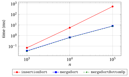
Figure 18.1: Measured running times of the three sorting algorithms (logarithmic scales on both axes).

• In a plot with logarithmic scales on both axes a power \(n^k\) is a straight line with slope \(k\): the line of Insertion Sort has slope close to \(2\), the lines of Merge Sort slope slightly larger than \(1\).

18.7.3 Fibonacci: naive recursion versus iteration

\(n\)	\(F(n)\)	calls of fibonacciRec	fibonacciRec	fibonacciIt
\(20\)	\(6\,765\)	\(21\,891\)	\(0.00808\) ms	\(4.0\) ns
\(25\)	\(75\,025\)	\(242\,785\)	\(0.0699\) ms	\(4.8\) ns
\(30\)	\(832\,040\)	\(2\,692\,537\)	\(0.764\) ms	\(7.4\) ns
\(35\)	\(9\,227\,465\)	\(29\,860\,703\)	\(9.15\) ms	\(8.4\) ns
\(40\)	\(102\,334\,155\)	\(331\,160\,281\)	\(93.8\) ms	\(9.5\) ns

• The numbers of calls were counted with a counter in the code and coincide with \(2F(n+1)-1\) (Observation 18.4).

• When \(n\) increases by \(5\), the time of fibonacciRec is multiplied by a factor between about \(9\) and \(12\), in agreement with \(\varphi^5\approx 11.09\). The time of fibonacciIt remains of a few nanoseconds.

• Extrapolating with the factor \(\varphi\) per unit of \(n\) from the measured time for \(n=40\):

  • fibonacciRec\((50)\) needs about \(93.8\cdot\varphi^{10}\approx 11\,500\) ms, i.e., about \(12\) seconds;

  • fibonacciRec\((60)\) needs about \(93.8\cdot\varphi^{20}\) ms, i.e., about \(24\) minutes;

  • fibonacciRec\((100)\) needs about \(93.8\cdot\varphi^{60}\) ms, i.e., about \(10\,000\) years.

• The compiler optimizes the code (with -O2 it merges several levels of the recursion into a single function call), so the time per call, about \(93.8\) ms\(/331\,160\,281\approx 0.28\) ns, is smaller than one would expect: this changes the constant, not the exponential growth.

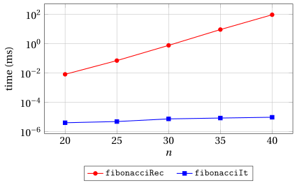
Figure 18.2: Measured running times of the recursive and of the iterative Fibonacci algorithms (logarithmic scale on the vertical axis).

• In a semi-logarithmic plot an exponential function is a straight line: the slope of the red line is about \(\log_{10}\varphi\approx 0.21\) per unit of \(n\).

18.7.4 Array sum: time and stack

\(n\)	sumIt	sumRecHalving	sumRecDecrease	sumRecDecrease, stack \(8\) MB
\(10^5\)	\(0.0215\) ms	\(0.0960\) ms	\(0.207\) ms	OK
\(10^6\)	\(0.210\) ms	\(0.910\) ms	\(2.24\) ms	crash
\(10^7\)	\(2.69\) ms	\(9.01\) ms	\(34.9\) ms	crash

• The three algorithms have the same order of growth \(\Theta(n)\): when \(n\) is multiplied by \(10\), all the times are multiplied by about \(10\) (between \(9.5\) and \(16\); from \(n=10^6\) to \(n=10^7\) the array no longer fits in the cache memory and the factors increase).

• The recursive versions are slower by a constant factor (about \(3\)–\(4.5\) for the halving version, about \(10\)–\(13\) for the decrease-by-one version): this is the call overhead.

• With the default stack of \(8\) MB, sumRecDecrease crashes (segmentation fault) for \(n=10^6\) and \(n=10^7\); the times of the table were measured by removing the limit with the command ulimit -s unlimited.

• By bisection on \(n\) (with a precision of \(10^3\)) we found that, with \(8\) MB, the largest \(n\) that does not crash is about \(6.97\cdot 10^5\) with -O2, and about \(2.62\cdot 10^5\) without optimization (-O0). Without optimization every call uses a frame of \(32\) bytes:

  \[ \frac{8\cdot 2^{20}}{32}=262\,144 . \]

  With -O2 the compiler merges four levels of the recursion into a single call with a frame of \(48\) bytes, so that

  \[ \frac{8\cdot 2^{20}}{48}\cdot 4\approx 6.99\cdot 10^5 : \]

  optimization changes the constant, not the \(\Theta(n)\) depth.

• sumRecHalving uses only \(\lceil\log_2 n\rceil+1\le 25\) frames for \(n\le 10^7\) and never crashes; sumIt uses no frame at all.

18.8 Guidelines

Use recursion when:

• the problem splits into a few independent subproblems of size \(n/b\) (divide and conquer), so that the Master Theorem gives a better running time than the iterative algorithms (Merge Sort, fast power, Karatsuba);

• the recursive description is the natural one and no asymptotic gain is possible anyway (Tower of Hanoi, and later visits of trees and graphs);

• the depth of the recursion is small, typically \(\Theta(\log_2 n)\).

Avoid recursion when:

• the problem only decreases from \(n\) to \(n-1\) with constant extra work: the recursion is a loop in disguise, with the same running time, a call overhead, \(\Theta(n)\) stack memory and a risk of stack overflow (factorial, linear sum, linear search);

• the subproblems overlap: the naive recursion repeats the same computations and can be exponential (Fibonacci); use memoization or, better, a bottom-up loop (Dynamic Programming).

Always consider the space: the call stack uses memory proportional to the depth of the recursion. Tail recursion can be eliminated mechanically, obtaining a loop with \(\Theta(1)\) extra memory.

Always compare with the best iterative algorithm: a recursive algorithm can improve on brute force and still be beaten by a smarter loop (Kadane's algorithm for the maximum subarray).

---

Exercises on this chapter: Recursive versus iterative algorithms