Linear and binary search
Part 1 · Basic algorithms · Chapter 4 · Lecture notes, volume 1 (PDF) · Exercises: Linear and binary search · App: Linear and binary search
4.1 The search problem
-
Looking for a value in a collection of data is one of the most frequent operations performed by a computer: a name in a list of contacts, a code in a table of products, a word in a dictionary.
-
In this chapter the collection is an array of natural numbers, and we present two algorithms that solve the problem:
-
linear search, which works on every array;
-
binary search, which works only on arrays sorted in non-decreasing order, but which is much faster than linear search on long arrays.
-
Definition 4.1: search problem
Given an array \(a[1..n]\) of \(n\) natural numbers and a target natural number \(m\), the search problem consists in determining if \(m\) is one of the elements of the array, i.e., if there exists an index \(k \in \{1, 2, \dots, n\}\) such that
An algorithm for the search problem returns such an index \(k\) if it exists, and the value \(-1\) otherwise.
- The value \(-1\) is never a valid index of the array \(a[1..n]\) (nor of a
C++array, whose indices start from \(0\)): for this reason it can be used to signal that the target value has not been found.
4.2 Linear search
Given an array \(a[1..n]\) of \(n\) natural numbers and a target natural number \(m\), we consider the problem of determining if \(m\) is one of the elements of the array.
-
The simplest idea is to compare the target \(m\) with the elements of the array one after the other, from the first to the last, and to stop as soon as an element equal to \(m\) is found.
-
This is the pseudo-code of the Linear Search algorithm that determines if a target value \(m\) is present in an array \(a[1..n]\) of \(n\) natural numbers:
Algorithm: LinearSearch
-
Explanation of the algorithm:
-
The algorithm scans the array sequentially from index \(1\) to \(n\).
-
At each iteration, it compares the element \(a[i]\) with the target \(m\) (line 4).
-
If \(a[i] = m\), the element is found and index \(i\) is returned (line 5).
-
If the loop completes without a match, the element is not in the array and \(-1\) is returned (line 9).
-
-
If \(m\) appears more than once in the array, the algorithm stops at the first match: the returned index is the smallest index \(k\) such that \(a[k]=m\).
Example 4.1: Linear Search
Consider the array \(a = [4, 2, 7, 1, 5, 9, 3]\) with \(n=7\).
-
Search for \(m = 5\):
iteration \(i\) \(a[i]\) action \(1\) 1 4 \(a[i] \neq m\) \(2\) 2 2 \(a[i] \neq m\) \(3\) 3 7 \(a[i] \neq m\) \(4\) 4 1 \(a[i] \neq m\) \(5\) 5 5 \(a[i] = m\) \(\Rightarrow\) Found! Accordingly, element 5 is found at index 5.
-
Search for \(m = 6\):
iteration \(i\) \(a[i]\) action \(1\) 1 4 \(a[i] \neq m\) \(2\) 2 2 \(a[i] \neq m\) \(3\) 3 7 \(a[i] \neq m\) \(4\) 4 1 \(a[i] \neq m\) \(5\) 5 5 \(a[i] \neq m\) \(6\) 6 9 \(a[i] \neq m\) \(7\) 7 3 \(a[i] \neq m\) \(-\) 8 \(-\) \(i > n\) \(\Rightarrow\) loop ends, Not found! Accordingly, element 6 is not in the array (return \(-1\)).
- The work done by linear search is measured by the number of comparisons \(a[i]=m\) at line 4: in the example, \(5\) comparisons are needed to find \(m=5\), and all the \(n=7\) elements are compared to conclude that \(m=6\) is not in the array.
Observation 4.2: number of comparisons of linear search
Given an array \(a[1..n]\) of \(n\) natural numbers and a target value \(m\):
Proof
The variable \(i\) takes the values \(1, 2, 3, \dots\) in this order, and at each value \(i \le n\) exactly one comparison \(a[i]=m\) is performed.
-
If \(k\) is the smallest index with \(a[k]=m\), then \(a[i] \neq m\) for \(i \in \{1, 2, \dots, k-1\}\), so the algorithm does not stop at these values of \(i\); for \(i=k\) the comparison is true and the algorithm returns \(k\). The comparisons are those with \(i = 1, 2, \dots, k\), i.e., \(k\) comparisons.
-
If \(m\) is not in the array, every comparison is false, so the loop is executed for \(i = 1, 2, \dots, n\) and stops when \(i = n+1\). The comparisons are \(n\), and the algorithm returns \(-1\) at line 9.
□
Linear search makes no assumption on the order of the elements. Its price is that, when the target is absent (or it is in the last position), all the \(n\) elements of the array must be examined.
4.3 Binary search
- Think of looking up a word in a paper dictionary: nobody reads it from the first page. We open it in the middle and, since the words are in alphabetical order, we know in which half to continue. Binary search applies the same idea to a sorted array.
Definition 4.3: sorted array
An array \(a[1..n]\) of \(n\) natural numbers is sorted in non-decreasing order if
Given an array \(a[1..n]\) of \(n\) natural numbers sorted in non-decreasing order and a target natural number \(m\), we consider the problem of determining if \(m\) is one of the elements of the array.
-
Binary search keeps a portion \(a[left..right]\) of the array, called the search interval, which is the only portion that may still contain \(m\). At the beginning the search interval is the whole array.
-
At each iteration the target \(m\) is compared with the element \(a[mid]\) in the middle of the search interval:
-
if \(a[mid] < m\), then, since the array is sorted, all the elements \(a[left], \dots, a[mid]\) are smaller than \(m\), and the search continues in the right half \(a[mid+1..right]\);
-
if \(a[mid] > m\), then all the elements \(a[mid], \dots, a[right]\) are greater than \(m\), and the search continues in the left half \(a[left..mid-1]\).
-
-
This is the pseudo-code of the Binary Search algorithm that determines if a target value \(m\) is present in an array \(a[1..n]\) of \(n\) natural numbers sorted in non-decreasing order:
Algorithm: BinarySearch
-
Explanation of the algorithm:
-
The algorithm maintains two indices, \(left\) and \(right\), defining the search interval \(a[left..right]\), which contains \(right-left+1\) elements.
-
At each iteration, it computes the middle index \(mid\) (line 5) and compares \(a[mid]\) with the target \(m\).
-
If \(a[mid] = m\), the element is found and its index is returned (line 7).
-
If \(a[mid] < m\), the search continues in the right half by updating \(left \leftarrow mid + 1\) (line 10).
-
If \(a[mid] > m\), the search continues in the left half by updating \(right \leftarrow mid - 1\) (line 13).
-
If the search interval becomes empty (\(left > right\)), the element is not in the array and \(-1\) is returned (line 16).
-
-
Since \(0 \le \lfloor (right-left)/2 \rfloor \le right-left\), the index \(mid\) always lies in the search interval: \(left \le mid \le right\).
Example 4.3: Binary Search
Consider the sorted array \(a = [3, 9, 11, 12, 12, 16, 19]\) with \(n=7\).
-
Search for \(m = 12\):
iteration \(left\) \(right\) \(mid\) \(a[mid]\) action \(1\) 1 7 4 12 \(a[mid] = m\) \(\Rightarrow\) Found! Accordingly, element 12 is found at index 4.
-
Search for \(m = 10\):
iteration \(left\) \(right\) \(mid\) \(a[mid]\) action \(1\) 1 7 4 12 \(a[mid] > m\) \(\Rightarrow\) \(right \leftarrow 3\) \(2\) 1 3 2 9 \(a[mid] < m\) \(\Rightarrow\) \(left \leftarrow 3\) \(3\) 3 3 3 11 \(a[mid] > m\) \(\Rightarrow\) \(right \leftarrow 2\) \(-\) 3 2 \(-\) \(-\) \(left > right\) \(\Rightarrow\) Not found! Accordingly, element 10 is not in the array (return \(-1\)).
-
Search for \(m = 3\):
iteration \(left\) \(right\) \(mid\) \(a[mid]\) action \(1\) 1 7 4 12 \(a[mid] > m\) \(\Rightarrow\) \(right \leftarrow 3\) \(2\) 1 3 2 9 \(a[mid] > m\) \(\Rightarrow\) \(right \leftarrow 1\) \(3\) 1 1 1 3 \(a[mid] = m\) \(\Rightarrow\) Found! Accordingly, element 3 is found at index 1.
-
Search for \(m = 19\):
iteration \(left\) \(right\) \(mid\) \(a[mid]\) action \(1\) 1 7 4 12 \(a[mid] < m\) \(\Rightarrow\) \(left \leftarrow 5\) \(2\) 5 7 6 16 \(a[mid] < m\) \(\Rightarrow\) \(left \leftarrow 7\) \(3\) 7 7 7 19 \(a[mid] = m\) \(\Rightarrow\) Found! Accordingly, element 19 is found at index 7.
- The following figure shows the search interval at each iteration of the search for \(m=10\): the elements outside the search interval (grey) are discarded, and the element \(a[mid]\) compared with \(m\) is highlighted in red.
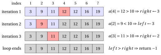
Figure 4.1: Search intervals of BinarySearch for \(m=10\) in \(a=[3, 9, 11, 12, 12, 16, 19]\): blue cells form the search interval \(a[left..right]\), the red cell is \(a[mid]\), grey cells have been discarded.
- If \(m\) appears more than once in the array, binary search returns the index of one of its occurrences, not necessarily the first one. For instance, for \(a=[1, 2, 2, 2, 2, 2, 3]\) and \(m=2\), the first iteration computes \(mid = 1 + \lfloor 6/2 \rfloor = 4\) and, since \(a[4] = 2 = m\), the algorithm returns \(4\), while
LinearSearchreturns \(2\).
4.3.1 Number of iterations
- Each iteration that does not find \(m\) discards the element \(a[mid]\) and at least half of the remaining elements of the search interval. This is why binary search is fast: the length of the search interval is (at least) halved at each iteration.
Observation 4.4: number of iterations of binary search
Given an array \(a[1..n]\) of \(n \ge 1\) natural numbers sorted in non-decreasing order and a target value \(m\), the while loop of BinarySearch executes at most
iterations.
Proof
Let \(L = right - left + 1 \ge 1\) be the number of elements of the search interval at the beginning of an iteration that does not return. Since \(mid = left + \lfloor (L-1)/2 \rfloor\), the new search interval has:
-
\(mid - left = \lfloor (L-1)/2 \rfloor\) elements, if \(right \leftarrow mid-1\);
-
\(right - mid = (L-1) - \lfloor (L-1)/2 \rfloor = \lceil (L-1)/2 \rceil\) elements, if \(left \leftarrow mid+1\).
In both cases the new number of elements is at most \(\lceil (L-1)/2 \rceil = \lfloor L/2 \rfloor \le L/2\).
At the beginning \(L = n\). Hence, after \(k\) iterations that do not return, the search interval has at most \(n/2^k\) elements. An iteration is executed only if the search interval is not empty, so iteration \(k+1\) is executed only if
Since \(k\) is an integer, \(k \le \lfloor \log_2 n \rfloor\), and the number \(k+1\) of any executed iteration is at most \(\lfloor \log_2 n \rfloor + 1\). □
-
In Example 4.3, \(n = 7\) and \(\lfloor \log_2 7 \rfloor + 1 = 3\): the searches for \(m=10\), \(m=3\) and \(m=19\) execute exactly \(3\) iterations, so the bound is attained.
-
The difference with linear search grows very quickly with \(n\). The following table compares the number of comparisons of linear search when \(m\) is not in the array (Observation 4.2) with the maximum number of iterations of binary search:
| \(n\) | linear search | binary search |
|---|---|---|
| \(n\) comparisons | at most \(\lfloor \log_2 n \rfloor + 1\) iterations | |
| \(1\,000\) | \(1\,000\) | \(10\) |
| \(1\,000\,000\) | \(1\,000\,000\) | \(20\) |
| \(1\,000\,000\,000\) | \(1\,000\,000\,000\) | \(30\) |
Binary search requires the array to be sorted in non-decreasing order. On a sorted array of \(n\) elements it executes at most \(\lfloor \log_2 n \rfloor + 1\) iterations, while linear search may need \(n\) comparisons. If the array is not sorted, binary search may wrongly discard the half that contains \(m\), and linear search must be used.
Key points of the chapter
-
The search problem asks for an index \(k\) such that \(a[k]=m\), or \(-1\) if no such index exists.
-
Linear search works on every array, returns the first occurrence of \(m\), and performs up to \(n\) comparisons.
-
Binary search works only on arrays sorted in non-decreasing order; it halves the search interval \(a[left..right]\) at each iteration and executes at most \(\lfloor \log_2 n \rfloor + 1\) iterations.
-
In the pseudo-code the indices go from \(1\) to \(n\), in the Colab notebooks (Python,
C++, Java) from \(0\) to \(n-1\): the returned indices differ by \(1\).
Exercises on this chapter: Linear and binary search
Interactive lab
The algorithm of the chapter, one step at a time: move the sliders and press ▶. The same graph full page, with the other ones of the course, is in the interactive lab.