Recursion

Part 5 · Recursion · Chapter 14 · Lecture notes, volume 5 (PDF) · Exercises: Recursion · App: Recursion trees

In the previous chapters every algorithm was iterative: a sequence of instructions and loops, whose number of steps we counted line by line (chapter «Running time») and whose correctness we proved with loop invariants (chapter «Correctness»). In this chapter we study a different way of designing algorithms: an algorithm may call itself on smaller instances of the same problem.

The plan of the chapter is the following.

• In Section 14.1 we define recursive algorithms, base cases and recursive steps, and we see why a recursive algorithm terminates.

• In Section 14.2 we describe how a recursive algorithm is executed: the tree of recursive calls (which determines the number of steps) and the call stack (which determines the memory).

• In Section 14.3 we show that the correctness of a recursive algorithm is proved by strong induction.

• In Sections 14.4–14.8 we apply these tools to five classical recursive algorithms: the factorial, the Fibonacci numbers, the greatest common divisor, fast exponentiation and the Towers of Hanoi. For each of them we prove the correctness, we count the number of steps by unrolling a recurrence; the implementations in Python, C++ and Java are in the Colab notebooks of the chapter.

14.1 Recursive algorithms

• Many problems have a natural self-similar structure: the solution of an instance can be easily obtained from the solution of one or more smaller instances of the same problem.

• For example, for every natural number \(n \ge 1\),

  \[ n! = n \cdot (n-1)! \]

  that is, the factorial of \(n\) is obtained from the factorial of the smaller number \(n-1\).

• Algorithms that exploit this structure are called recursive algorithms.

Definition 14.1: recursive algorithm

A recursive algorithm is an algorithm that solves an instance of a problem by calling itself on one or more smaller instances of the same problem, and then combining the results of these calls.

• Every recursive algorithm is made of two parts:

  1. Base case(s): one or more instances that are small enough to be solved directly, without any recursive call (for example, \(0! = 1\)).

  2. Recursive step: on every other instance, the algorithm calls itself on smaller instances and combines the returned results (for example, \(n! = n \cdot (n-1)!\)).

• Each execution of the algorithm on a given input is called a call (or invocation). A call that is made from inside another call is a recursive call.

• To measure how “small” an instance is, we associate to each input a size, which is a natural number (for example the value \(n\) of the input number, or the number \(n\) of entries of an array \(a[1..n]\)).

14.1.1 Termination

• A recursive algorithm terminates only if the chain of recursive calls eventually reaches a base case.

• If the size of the instance strictly decreases at each recursive call, we obtain a strictly decreasing sequence of natural numbers

  \[ n_0 > n_1 > n_2 > \cdots \]

• There is no infinite strictly decreasing sequence of natural numbers (by the well-ordering property of \(\N\)): after at most \(n_0\) calls the size cannot decrease anymore. Therefore, if every instance which is not a base case is reduced to strictly smaller instances, a base case is necessarily reached after finitely many calls.

Key idea of recursion.

• Solve the base cases directly.

• Reduce every other instance to one or more strictly smaller instances of the same problem, solve them by recursive calls, and combine their results.

• Since the size is a natural number that strictly decreases at every recursive call, a base case is always reached and the algorithm terminates.

Example 14.1: What can go wrong

• Missing base case. Consider the function WrongFactorial\((n)\) that returns \(n \cdot \texttt{WrongFactorial}(n-1)\), without any base case. The call WrongFactorial\((2)\) calls WrongFactorial\((1)\), which calls WrongFactorial\((0)\), which calls WrongFactorial\((-1)\), and so on forever: the recursion never stops.

• Size not decreasing. A function that, on input \(n\), calls itself on input \(n\) (or \(n+1\)) never reaches a base case \(n=0\) when \(n \ge 1\).

• In practice, an infinite recursion is stopped by the computer when the memory reserved to the calls is exhausted (a stack overflow error).

• To count the number of steps of a recursive algorithm we use the same conventions as in the chapter «Running time»: each execution of a line of pseudo-code is one step. A line that contains a recursive call counts as one step plus all the steps executed by that recursive call.

• As a consequence, the number of steps \(S(n)\) of a recursive algorithm is naturally expressed in terms of the number of steps on smaller instances, i.e., by a recurrence, such as

  \[ S(n) = S(n-1) + 2. \]

In this chapter we solve the recurrences of the step counts by simple unrolling (also called expansion): we replace repeatedly \(S(\cdot)\) by its definition until we reach a base case.

14.2 Tree of recursive calls and call stack

14.2.1 Tree of recursive calls

Definition 14.2: tree of recursive calls

The tree of recursive calls of a recursive algorithm on a given input is the rooted tree in which:

• every node is a call of the algorithm;

• the root is the initial call;

• the children of a node are the recursive calls made directly by that call, from left to right in the order in which they are executed.

The leaves of the tree are the calls that do not make recursive calls (typically the base cases).

• The total number of calls executed by the algorithm is the number of nodes of the tree.

• If every call executes a constant number of steps (excluding the steps of its recursive calls), then the number of steps of the algorithm is proportional to the number of nodes of the tree.

• The calls are executed following a depth-first visit of the tree: a call starts, executes its first recursive call (and the whole subtree below it) completely, then its second recursive call, and so on; it returns its result only when all its recursive calls have returned.

Example 14.2: Two shapes of trees of recursive calls

• If each call makes one recursive call (as for \(n! = n\cdot(n-1)!\)), the tree is a path (left).

• If each call makes two recursive calls (as for the Fibonacci numbers, defined by \(F(n) = F(n-1)+F(n-2)\) with \(F(0)=0\) and \(F(1)=1\)), the tree branches and the number of nodes can grow very quickly (right).

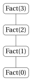
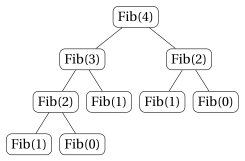
14.2.2 Call stack

• When a call starts, the computer reserves a piece of memory, called a stack frame (or activation record), that contains the parameters of the call, its local variables, and the point of the program where the execution must continue when the call returns.

• The frames are stored in a memory area organised as a stack (the call stack):

  • when a call starts, its frame is pushed on top of the stack;

  • when a call returns, its frame is popped from the top of the stack, and the execution continues in the call whose frame is now on top.

• At any moment, the frames in the stack are exactly the calls on the path from the root of the tree of recursive calls to the call currently executed.

Definition 14.3: depth of the recursion

The depth of the recursion of a recursive algorithm on a given input is the maximum number of calls that are simultaneously active, i.e., the maximum number of nodes on a path from the root to a leaf of the tree of recursive calls.

The maximum number of stack frames simultaneously in memory is equal to the depth of the recursion. If every frame uses a constant amount of memory, the memory used by the call stack is

\[ \Theta(\text{depth of the recursion}). \]

• Note the difference: the number of steps depends on the number of nodes of the tree, while the memory used by the call stack depends only on its depth.

• For the tree of Fib(4) above, there are \(9\) calls, but at most \(4\) of them are simultaneously in the stack (for example Fib(4), Fib(3), Fib(2), Fib(1)).

Example 14.3: Evolution of the call stack for Fact(3)

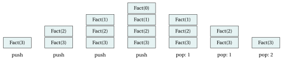
The figure shows the call stack (top of the stack is up) after each push and after each pop, during the computation of \(3!\) with the recursion \(n! = n \cdot (n-1)!\), \(0!=1\).

• Four frames are pushed: Fact(3), Fact(2), Fact(1), Fact(0).

• Fact(0) is a base case: it returns \(1\) and its frame is popped. Then Fact(1) returns \(1\cdot 1 = 1\), Fact(2) returns \(2 \cdot 1 = 2\) and, finally, Fact(3) returns \(3 \cdot 2 = 6\) and the stack becomes empty.

• The depth of the recursion is \(4\).

• The size of the call stack is limited (typically a few megabytes). A very deep recursion (for example, millions of nested calls) causes a stack overflow, even if the algorithm is correct and terminates.

14.3 Correctness of recursive algorithms

• The natural tool to prove the correctness of a recursive algorithm is mathematical induction on the size of the input.

• Since a recursive call can be made on any smaller instance (not only on the instance of size \(n-1\)), we use strong induction.

Strong induction. Let \(P(n)\) be a statement depending on \(n \in \N\), and let \(n_0 \in \N\). If

1. base case: \(P(n_0)\) is true, and

2. inductive step: for every \(n > n_0\), if \(P(k)\) is true for every \(k\) with \(n_0 \le k < n\) (inductive hypothesis), then \(P(n)\) is true,

then \(P(n)\) is true for every natural number \(n \ge n_0\).

• It is sometimes convenient to prove more than one base case (for example \(n=0\) and \(n=1\)), and then the inductive step only for \(n\) larger than all of them.

• The structure of a recursive algorithm mirrors the structure of an induction proof:

  • the base cases of the algorithm correspond to the base cases of the induction;

  • in the recursive step, we may assume (inductive hypothesis) that the recursive calls, which are made on smaller inputs, return correct results, and we only need to show that the results are combined correctly.

Observation 14.4: correctness of recursive algorithms

Consider a recursive algorithm in which every input has a size in \(\N\). Assume that:

1. on every input which is a base case, the algorithm returns the correct output;

2. on every other input of size \(n\), the algorithm makes a finite number of recursive calls, all on inputs of size strictly smaller than \(n\), and returns the correct output whenever all these recursive calls return the correct output.

Then the algorithm terminates and returns the correct output on every input.

Proof

Let \(P(n)\) be the statement: “on every input of size \(n\) the algorithm terminates and returns the correct output”. We prove \(P(n)\) for every \(n \in \N\) by strong induction.

Let \(n \in \N\) and assume that \(P(k)\) is true for every \(k < n\) (for \(n=0\) this assumption is empty). Consider an input of size \(n\).

• If the input is a base case, then the algorithm terminates and returns the correct output by hypothesis 1.

• Otherwise, by hypothesis 2, the algorithm makes a finite number of recursive calls on inputs of size \(k < n\). By the inductive hypothesis, each of these calls terminates and returns the correct output. Hence the algorithm terminates and, by hypothesis 2, it returns the correct output.

Therefore \(P(n)\) is true, and by strong induction \(P(n)\) is true for every \(n \in \N\). □

14.3.1 Link with loop invariants

• In the chapter «Correctness» we proved the correctness of iterative algorithms by means of loop invariants, which also have the structure of an induction proof.

• The three properties of a loop invariant correspond to the parts of the proof by induction of a recursive algorithm:

Loop invariant (iterative algorithm)	Induction (recursive algorithm)
Initialization: true before the first iteration	Base case(s) of the recursion
Maintenance: preserved by each iteration	Inductive step: correct combination of the results
Termination: the loop stops	The size strictly decreases towards a base case

• The main difference is the direction: an iterative algorithm builds the solution “from the bottom” (from the initialization towards the final iteration), while a recursive algorithm starts “from the top” (the original instance) and reduces it to smaller instances until a base case is reached.

14.4 Factorial

Given a natural number \(n\), we consider the problem of computing the factorial of \(n\):

\[ n! = 1 \cdot 2 \cdot \ldots \cdot n \qquad \text{with } 0! = 1. \]

• Since \(n! = n \cdot (n-1)!\) for every \(n \ge 1\), the factorial has the following recursive definition:

  \[ n! = \begin{cases} 1 & \text{if } n = 0 \\ n \cdot (n-1)! & \text{if } n \ge 1 \end{cases} \]

• This is the pseudo-code of the recursive algorithm Factorial:

Algorithm: Factorial

Input: A natural number \(n\)

Output: The factorial \(n!\)

1function Factorial(n)

2if \(n = 0\) then

3return \(1\)// base case

4end

5return \(n \cdot\) Factorial\((n-1)\)// recursive step

6end

Run in Colab:PythonC++Java

• Explanation of the algorithm:

  • The base case is \(n=0\), for which the algorithm returns \(0! = 1\).

  • For \(n \ge 1\), the algorithm calls itself on the smaller input \(n-1\) and multiplies the result by \(n\).

  • The size of the input is the value \(n\), which decreases by one at each recursive call. Hence the base case is reached after \(n\) recursive calls.

Example 14.4: Tree of recursive calls of Factorial(4)

The tree is a path with \(5\) nodes. The value returned by each call is written in red next to the call.

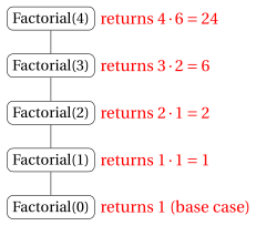
The calls are made from the top to the bottom; the results are returned from the bottom to the top. The depth of the recursion is \(5\).

14.4.1 Correctness

Observation 14.5: correctness of Factorial

For every natural number \(n\), the call Factorial\((n)\) terminates and returns \(n!\).

Proof

We proceed by induction on \(n\).

• Base case (\(n=0\)): the condition of line 2 is true and the algorithm returns \(1 = 0!\) at line 3.

• Inductive step (\(n \ge 1\)): assume that Factorial\((n-1)\) terminates and returns \((n-1)!\) (inductive hypothesis). Since \(n \ne 0\), the algorithm executes line 5 and returns

  \[ n \cdot \texttt{Factorial}(n-1) = n \cdot (n-1)! = n!. \]

Therefore Factorial\((n)\) returns \(n!\) for every \(n \in \N\). □

14.4.2 Number of steps

• Let \(S(n)\) denote the number of steps executed by Factorial on the input \(n\) (there is only one input for each value of \(n\), so this is also the worst case).

• If \(n = 0\), lines 2 and 3 are executed once each:

  \[ S(0) = 2. \]

• If \(n \ge 1\), lines 2 and 5 are executed once each, and line 5 also executes all the steps of the call Factorial\((n-1)\):

  \[ S(n) = S(n-1) + 2. \]

• We solve the recurrence by unrolling it:

  \[\begin{align*} S(n) &= S(n-1) + 2 \\ &= \big(S(n-2) + 2\big) + 2 = S(n-2) + 2\cdot 2 \\ &= \big(S(n-3) + 2\big) + 2 \cdot 2 = S(n-3) + 3 \cdot 2 \\ &\;\;\vdots \\ &= S(n-k) + k \cdot 2 \qquad \forall k \in \{1, 2, \dots, n\}. \end{align*}\]

  Choosing \(k = n\) (base case), we obtain

  \[ S(n) = S(0) + 2n = 2n + 2. \]

• Therefore,

  \[ S(n) = 2n + 2 = \Theta(n), \]

  since

  \[ \lim_{n \to \infty} \frac{2n+2}{n} = \lim_{n \to \infty} \left(2 + \frac{2}{n}\right) = 2 \in \R_{>0}. \]

• The depth of the recursion is \(n+1\) (the calls with inputs \(n, n-1, \dots, 0\) are all simultaneously in the stack), so the call stack uses \(\Theta(n)\) memory. The iterative algorithm that computes \(n!\) with a while loop uses only a constant amount of memory.

• We now express the number of steps as a function of the input size \(|I|\). As in the chapter «Running time», we count each multiplication as one step. The input is the natural number \(n\), which requires \(\lfloor \log_2 n\rfloor + 1\) bits (for \(n \ge 1\)), hence

  \[ |I| = \Theta(\log_2 n). \]

  This means that there exist constants \(c_1, c_2 > 0\) such that, for all sufficiently large \(n\),

  \[ c_1 \log_2 n \le |I| \le c_2 \log_2 n \qquad \Longleftrightarrow \qquad 2^{\frac{1}{c_2}|I|} \le n \le 2^{\frac{1}{c_1}|I|}. \]

  Since \(S(n) = \Theta(n)\), there exist constants \(a_1, a_2 > 0\) such that \(a_1 n \le S(n) \le a_2 n\) for all sufficiently large \(n\), and therefore

  \[ a_1 2^{\frac{1}{c_2}|I|} \le S(n) \le a_2 2^{\frac{1}{c_1}|I|}, \]

  that is, \(T(|I|) = 2^{\Theta(|I|)}\).

The number of steps of the Factorial algorithm is \(S(n) = 2n+2 = \Theta(n)\), and its depth of recursion is \(n+1\). As a function of the input size \(|I| = \Theta(\log_2 n)\), the worst-case running time is

\[ T(|I|) = 2^{\Theta(|I|)}, \]

i.e., it is linear in the numerical value \(n\), but exponential in the input size \(|I|\).

14.5 Fibonacci numbers

Given a natural number \(n\), we consider the problem of computing the \(n\)-th Fibonacci number \(F(n)\), defined as

\[ F(n) = \begin{cases} n & \text{if } n \in \{0, 1\} \\ F(n-1) + F(n-2) & \text{if } n \ge 2 \end{cases} \]

• The first Fibonacci numbers are:

  \(n\)	0	1	2	3	4	5	6	7	8	9	10
  \(F(n)\)	0	1	1	2	3	5	8	13	21	34	55

• The definition is itself recursive, and it directly gives the following (naive) recursive algorithm Fib, with two base cases and two recursive calls:

Algorithm: Fib

Input: A natural number \(n\)

Output: The Fibonacci number \(F(n)\)

1function Fib(n)

2if \(n \le 1\) then

3return \(n\)// base cases

4end

5return Fib\((n-1)\) \(+\) Fib\((n-2)\)// recursive step

6end

Run in Colab:PythonC++Java

Observation 14.6: correctness of Fib

For every natural number \(n\), the call Fib\((n)\) terminates and returns \(F(n)\).

Proof

We proceed by strong induction on \(n\).

• Base cases (\(n \in \{0,1\}\)): the algorithm returns \(n = F(n)\) at line 3.

• Inductive step (\(n \ge 2\)): by the inductive hypothesis the two calls on the smaller inputs \(n-1\) and \(n-2\) return \(F(n-1)\) and \(F(n-2)\), and line 5 returns their sum \(F(n)\).

Here two base cases are needed, because the inductive step for \(n\) uses both \(n-1\) and \(n-2\). □

Example 14.6: Tree of recursive calls of Fib(5)

Each node is a call; the value returned by the call is written in red below it.

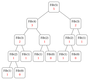
• The tree has \(15\) nodes: the algorithm makes \(15\) calls to compute \(F(5) = 5\).

• The same subproblems are solved many times: Fib(3) is computed \(2\) times, Fib(2) \(3\) times, Fib(1) \(5\) times and Fib(0) \(3\) times.

• The depth of the recursion is \(5\) (for example, the path Fib(5), Fib(4), Fib(3), Fib(2), Fib(1)).

14.5.1 Number of calls and number of steps

• Let \(C(n)\) denote the number of calls (nodes of the tree) executed by Fib\((n)\). Each call with \(n \ge 2\) generates one call on \(n-1\) and one call on \(n-2\), hence

  \[ C(n) = \begin{cases} 1 & \text{if } n \in \{0, 1\} \\ C(n-1) + C(n-2) + 1 & \text{if } n \ge 2 \end{cases} \]

• The first values are \(C(0)=1\), \(C(1)=1\), \(C(2)=3\), \(C(3)=5\), \(C(4)=9\), \(C(5)=15\), \(C(6)=25\). They are related to the Fibonacci numbers themselves:

Observation 14.7: number of calls of Fib

For every natural number \(n\),

\[ C(n) = 2F(n+1) - 1. \]

Proof

We proceed by strong induction on \(n\).

• Base cases: \(C(0) = 1 = 2 \cdot 1 - 1 = 2F(1) - 1\) and \(C(1) = 1 = 2 \cdot 1 - 1 = 2F(2) - 1\).

• Inductive step (\(n \ge 2\)): assume \(C(k) = 2F(k+1)-1\) for every \(k < n\). Then

  \[\begin{align*} C(n) &= C(n-1) + C(n-2) + 1 \\ &= \big(2F(n) - 1\big) + \big(2F(n-1) - 1\big) + 1 \\ &= 2\big(F(n) + F(n-1)\big) - 1 = 2F(n+1) - 1. \end{align*}\]

□

• For example, \(C(5) = 2F(6) - 1 = 2 \cdot 8 - 1 = 15\), as in Example 14.6.

• Each call executes exactly \(2\) lines (lines 2–3 for a base case, lines 2 and 5 otherwise), hence the number of steps \(S(n)\) satisfies

  \[ S(n) = S(n-1) + S(n-2) + 2 \quad (n \ge 2), \qquad S(0) = S(1) = 2, \]

  and therefore \(S(n) = 2C(n) = 4F(n+1) - 2\).

• The number of calls grows exponentially in \(n\):

Observation 14.8: exponential number of calls of Fib

For every natural number \(n \ge 2\),

\[ 2^{n/2} \le C(n) \le 2^n. \]

Proof

Lower bound. We proceed by strong induction on \(n \ge 2\).

• Base cases: \(C(2) = 3 \ge 2 = 2^{2/2}\) and \(C(3) = 5 \ge 2\sqrt{2} = 2^{3/2}\).

• Inductive step (\(n \ge 4\)): assume the claim for every \(k\) with \(2 \le k < n\); in particular for \(k = n-2 \ge 2\). Since \(C(n-1) \ge C(n-2)\) (the sequence \(C\) is non-decreasing),

  \[ C(n) = C(n-1) + C(n-2) + 1 > 2\,C(n-2) \ge 2 \cdot 2^{(n-2)/2} = 2^{n/2}. \]

Upper bound. Also by strong induction: \(C(2) = 3 \le 4\), \(C(3) = 5 \le 8\) and, for \(n \ge 4\),

\[ C(n) = C(n-1) + C(n-2) + 1 \le 2^{n-1} + 2^{n-2} + 2^{n-2} = 2^n, \]

where we used \(1 \le 2^{n-2}\). □

• Note that \(C(1) = 1 < 2^{1/2}\): this is why the lower bound is stated for \(n \ge 2\).

• Therefore \(S(n) = 2C(n) = 2^{\Theta(n)}\): the naive recursive algorithm is exponential in \(n\). For example, the computation of \(F(30) = 832040\) requires \(C(30) = 2F(31) - 1 = 2 \cdot 1346269 - 1 = 2692537\) calls.

• (It can be shown that \(F(n)\) grows as \(\varphi^n/\sqrt{5}\), where \(\varphi = \frac{1+\sqrt{5}}{2} \approx 1.618\) is the golden ratio; hence \(C(n) = \Theta(\varphi^n)\).)

14.5.2 An iterative algorithm

• The reason of the exponential number of calls is that the naive algorithm solves the same subproblems again and again (see Example 14.6). An iterative algorithm computes each Fibonacci number only once, from \(F(0)\) and \(F(1)\) upwards, keeping only the last two values:

Algorithm: IterativeFib

Input: A natural number \(n\)

Output: The Fibonacci number \(F(n)\)

1function IterativeFib(n)

2if \(n \le 1\) then

3return \(n\)

4end

5\(prev := 0\)

6\(curr := 1\)

7\(i := 2\)

8while \(i \le n\) do

9\(next := prev + curr\)

10\(prev \leftarrow curr\)

11\(curr \leftarrow next\)

12\(i \leftarrow i + 1\)

13end

14return \(curr\)

15end

Run in Colab:PythonC++Java

• For \(n \ge 2\): lines 2, 5, 6, 7, 14 are executed once, line 8 is executed \(n\) times and lines 9–12 are executed \(n-1\) times. Hence

  \[ S(n) = 5 + n + 4(n-1) = 5n + 1 = \Theta(n). \]

• (Loop invariant: before each test of line 8, \(prev = F(i-2)\) and \(curr = F(i-1)\); at the end \(i = n+1\) and \(curr = F(n)\).)

\(n\)	\(F(n)\)	steps of Fib: \(4F(n+1)-2\)	steps of IterativeFib: \(5n+1\)
\(5\)	\(5\)	\(30\)	\(26\)
\(10\)	\(55\)	\(354\)	\(51\)
\(20\)	\(6765\)	\(43782\)	\(101\)
\(30\)	\(832040\)	\(5385074\)	\(151\)

The naive recursive algorithm Fib executes \(S(n) = 4F(n+1) - 2 = 2^{\Theta(n)}\) steps (exponential in \(n\)), while IterativeFib executes \(S(n) = 5n+1 = \Theta(n)\) steps (linear in \(n\)). Since \(|I| = \Theta(\log_2 n)\), as functions of the input size the naive algorithm is even doubly exponential, while the iterative one is exponential (as Factorial).

• The recursion itself is not the problem: the problem is the repetition of identical subproblems. Storing the solution of each subproblem the first time it is solved, and reusing it afterwards, is the key idea of the technique called Dynamic Programming.

14.6 Greatest common divisor

Given two natural numbers \(n, m\) with \(n \ge 1\) and \(m \ge 0\), we consider the problem of computing their greatest common divisor \(\gcd(n,m)\) (with \(\gcd(n,0) = n\)).

• In the chapter «Numerical algorithms» we proved that, for all natural numbers \(n \ge 1\) and \(m \ge 1\),

  \[ \gcd(n,m) = \gcd(m,\ n \bmod m), \]

  and we obtained the iterative algorithm EuclideanAlgorithm: it replaces the pair \((n,m)\) by the pair \((m,\ n \bmod m)\) again and again, until \(m = 0\).

• The same property, together with \(\gcd(n,0) = n\), is a recursive definition:

  \[ \gcd(n,m) = \begin{cases} n & \text{if } m = 0 \\ \gcd(m,\ n \bmod m) & \text{if } m \ge 1 \end{cases} \]

• This gives the recursive version of the Euclidean algorithm:

Algorithm: RecursiveGCD

Input: Two natural numbers \(n \ge 1\) and \(m \ge 0\)

Output: \(\gcd(n,m)\)

1function RecursiveGCD(n, m)

2if \(m = 0\) then

3return \(n\)// base case

4end

5return RecursiveGCD\((m,\ n \bmod m)\)// recursive step

6end

Run in Colab:PythonC++Java

• The size of the input is the second argument \(m\). Since \(0 \le n \bmod m < m\), the second argument strictly decreases at each recursive call, hence the base case \(m = 0\) is always reached.

Example 14.8: Trees of recursive calls of RecursiveGCD

Each call makes at most one recursive call, so the trees are paths.

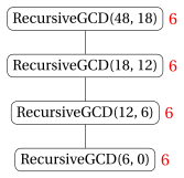
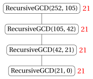
• \(48 \bmod 18 = 12\), \(18 \bmod 12 = 6\), \(12 \bmod 6 = 0\): hence \(\gcd(48,18) = 6\).

• \(252 \bmod 105 = 42\), \(105 \bmod 42 = 21\), \(42 \bmod 21 = 0\): hence \(\gcd(252,105) = 21\).

• The value found by the base case is returned unchanged by all the calls.

14.6.1 Correctness

Observation 14.9: correctness of RecursiveGCD

For every pair of natural numbers \(n \ge 1\) and \(m \ge 0\), the call RecursiveGCD\((n,m)\) terminates and returns \(\gcd(n,m)\).

Proof

We proceed by strong induction on \(m\).

• Base case (\(m = 0\)): the algorithm returns \(n = \gcd(n, 0)\) at line 3.

• Inductive step (\(m \ge 1\)): assume the claim for every second argument \(k < m\) and every first argument \(\ge 1\). The algorithm calls RecursiveGCD\((m,\ n \bmod m)\), where \(m \ge 1\) and \(n \bmod m < m\). By the inductive hypothesis, this call returns \(\gcd(m,\ n \bmod m)\), which is equal to \(\gcd(n,m)\) by the property \(\gcd(n,m) = \gcd(m,\ n \bmod m)\) recalled at the beginning of this section.

□

14.6.2 Tail recursion

Definition 14.10: tail recursion

A recursive call is a tail call if it is the last operation executed by the calling function, and its result is returned unchanged. A recursive algorithm whose recursive calls are all tail calls is tail recursive.

• RecursiveGCD is tail recursive: line 5 returns directly the result of the recursive call, without any further operation.

• Factorial is not tail recursive: after the recursive call Factorial\((n-1)\) returns, the result must still be multiplied by \(n\), so the frame of the caller must be kept in the stack.

A tail-recursive algorithm can always be transformed into a while loop: the tail call is replaced by the update of the parameters, and the loop continues until the base case is reached. Applying this transformation to RecursiveGCD, with the update \((n,m) \leftarrow (m,\ n \bmod m)\), we obtain exactly the iterative EuclideanAlgorithm, which uses a constant amount of memory. Many compilers apply this transformation automatically (tail-call optimization).

14.6.3 Number of steps

• Each call executes exactly \(2\) lines (lines 2–3, or lines 2 and 5), so the number of steps is twice the number of calls. We bound the number of calls.

• Let \(m_0 = m\) and let \(m_0, m_1, m_2, \dots, m_K = 0\) be the second arguments of the successive calls. The call \(k \ge 1\) is RecursiveGCD\((m_{k-1}, m_k)\) and therefore

  \[ m_{k+1} = m_{k-1} \bmod m_k, \qquad m_{k+1} < m_k. \]

Observation 14.11: the second argument halves every two calls

For every \(k\) such that \(m_{k+2}\) is defined,

\[ m_{k+2} < \frac{m_k}{2}. \]

Proof

We have \(m_{k+2} = m_k \bmod m_{k+1}\) with \(m_{k+1} < m_k\). We distinguish two cases.

• If \(m_{k+1} \le m_k/2\), then \(m_{k+2} < m_{k+1} \le m_k / 2\).

• If \(m_{k+1} > m_k/2\), then \(m_k < 2m_{k+1}\), so the quotient of \(m_k\) divided by \(m_{k+1}\) is \(1\) and \(m_{k+2} = m_k - m_{k+1} < m_k - m_k/2 = m_k/2\).

□

• Let \(m \ge 1\) and \(j = \lfloor \log_2 m \rfloor + 1\), so that \(2^j > m\). Applying the Observation \(j\) times, if \(m_{2j}\) is defined then

  \[ m_{2j} < \frac{m}{2^j} < 1 \quad \Longrightarrow \quad m_{2j} = 0. \]

  Hence \(K \le 2j\) and the number of calls (\(K+1\)) is at most \(2\lfloor \log_2 m \rfloor + 3\). Therefore

  \[ S(n,m) \le 2\big(2\lfloor \log_2 m \rfloor + 3\big) = O(\log_2 m). \]

• The input consists of the two numbers \(n\) and \(m\), so \(|I| = \Omega(\log_2 m)\) (for \(m \ge 2\)) and, as for ChangeToBase2 in the chapter «Running time», \(S(n,m) = O(|I|)\).

The RecursiveGCD algorithm makes at most \(2\lfloor \log_2 m \rfloor + 3\) calls, and its worst-case running time is

\[ T(|I|) = O(|I|), \]

i.e., it is at most linear in the input size. (It can be shown that the worst case occurs for two consecutive Fibonacci numbers: for example \(\gcd(89, 55)\) requires \(10\) calls, against the bound \(2\lfloor \log_2 55 \rfloor + 3 = 13\).)

14.7 Fast exponentiation

Given a number \(x\) and a natural number \(n\), we consider the problem of computing the power \(x^n\) (with \(x^0 = 1\)).

• The naive algorithm multiplies \(n\) times by \(x\):

  \[ p := 1, \qquad p \leftarrow p \cdot x \quad (n \text{ times}), \]

  which requires \(n\) multiplications and \(\Theta(n)\) steps.

• A much faster algorithm is obtained by squaring. Since \(n = 2\lfloor n/2 \rfloor\) if \(n\) is even, and \(n = 2\lfloor n/2 \rfloor + 1\) if \(n\) is odd,

  \[ x^n = \begin{cases} 1 & \text{if } n = 0 \\ \left(x^{\lfloor n/2 \rfloor}\right)^2 & \text{if } n \ge 1 \text{ is even} \\ x \cdot \left(x^{\lfloor n/2 \rfloor}\right)^2 & \text{if } n \text{ is odd} \end{cases} \]

  (for \(n\) odd, \(\lfloor n/2 \rfloor = (n-1)/2\)). The size of the exponent is halved at each recursive call.

Algorithm: FastPower

Input: A number \(x\) and a natural number \(n\)

Output: The power \(x^n\)

1function FastPower(x, n)

2if \(n = 0\) then

3return \(1\)// base case

4end

5\(y :=\) FastPower\((x, \lfloor n/2 \rfloor)\)// one recursive call

6if \(n \bmod 2 = 0\) then

7return \(y \cdot y\)// \(n\) even

8else

9return \(x \cdot y \cdot y\)// \(n\) odd

10end

11end

Run in Colab:PythonC++Java

• Note that the result of the recursive call is stored in the variable \(y\) and used twice: writing FastPower\((x, \lfloor n/2 \rfloor) \cdot\) FastPower\((x, \lfloor n/2 \rfloor)\) would make two identical recursive calls and would destroy the efficiency of the algorithm (this variant is analysed in the exercises of the chapter).

Example 14.10: Tree of recursive calls of FastPower(x, 13)

The exponents of the calls are \(13, 6, 3, 1, 0\) (\(\lfloor 13/2 \rfloor = 6\), \(\lfloor 6/2 \rfloor = 3\), \(\lfloor 3/2 \rfloor = 1\), \(\lfloor 1/2 \rfloor = 0\)). On the right of each call: the value returned and the number of multiplications executed by that call.

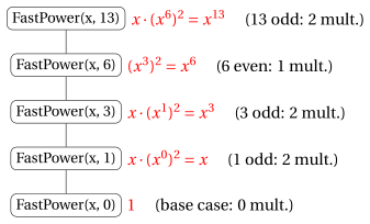
• Total number of multiplications: \(2 + 1 + 2 + 2 + 0 = 7\), against the \(13\) multiplications of the naive algorithm.

• Note that \(13 = (1101)_2\): the odd/even exponents met going up from FastPower\((x,1)\) to FastPower\((x,13)\) (odd, odd, even, odd) are exactly the binary digits \(1,1,0,1\) of \(13\) read from the most significant one. In general, the number of multiplications is the number of binary digits of \(n\) plus the number of digits equal to \(1\): here \(4 + 3 = 7\).

14.7.1 Correctness

Observation 14.12: correctness of FastPower

For every number \(x\) and every natural number \(n\), the call FastPower\((x,n)\) terminates and returns \(x^n\).

Proof

We proceed by strong induction on \(n\).

• Base case (\(n=0\)): the algorithm returns \(1 = x^0\) at line 3.

• Inductive step (\(n \ge 1\)): assume that FastPower\((x,k)\) returns \(x^k\) for every \(k < n\). Since \(n \ge 1\), we have \(\lfloor n/2 \rfloor < n\), so by the inductive hypothesis line 5 assigns \(y = x^{\lfloor n/2 \rfloor}\).

  • If \(n\) is even, then \(n = 2\lfloor n/2 \rfloor\) and line 7 returns \(y \cdot y = x^{2\lfloor n/2 \rfloor} = x^n\).

  • If \(n\) is odd, then \(n = 2\lfloor n/2 \rfloor + 1\) and line 9 returns \(x \cdot y \cdot y = x^{2\lfloor n/2 \rfloor + 1} = x^n\).

Note that strong induction is needed: the inductive hypothesis is used for \(k = \lfloor n/2 \rfloor\), not for \(k = n-1\). □

14.7.2 Number of steps

• Let \(S(n)\) denote the number of steps of FastPower on the exponent \(n\). If \(n = 0\), lines 2–3 are executed: \(S(0) = 2\). If \(n \ge 1\), lines 2, 5, 6 and one of the lines 7, 9 are executed once each, plus the steps of the call on \(\lfloor n/2 \rfloor\):

  \[ S(n) = S(\lfloor n/2 \rfloor) + 4 \qquad (n \ge 1). \]

• We solve the recurrence by unrolling it. Since \(\big\lfloor \lfloor n/2^{k} \rfloor / 2 \big\rfloor = \lfloor n/2^{k+1} \rfloor\),

  \[\begin{align*} S(n) &= S(\lfloor n/2 \rfloor) + 4 \\ &= S(\lfloor n/4 \rfloor) + 2 \cdot 4 \\ &\;\;\vdots \\ &= S(\lfloor n/2^k \rfloor) + k \cdot 4, \end{align*}\]

  as long as \(\lfloor n/2^{k-1} \rfloor \ge 1\). Now \(\lfloor n/2^k \rfloor \ge 1\) if and only if \(2^k \le n\), i.e., \(k \le \lfloor \log_2 n \rfloor\). Hence, for \(n \ge 1\), the exponents \(n, \lfloor n/2 \rfloor, \dots, \lfloor n/2^{\lfloor \log_2 n \rfloor}\rfloor = 1\) are all \(\ge 1\), and the next one is \(0\). Choosing \(k = \lfloor \log_2 n \rfloor + 1\):

  \[ S(n) = S(0) + 4\big(\lfloor \log_2 n \rfloor + 1\big) = 4\lfloor \log_2 n \rfloor + 6. \]

• For example, \(S(13) = 4 \cdot 3 + 6 = 18\). As shown for ChangeToBase2 in the chapter «Running time»,

  \[ \lim_{n \to \infty} \frac{4\lfloor \log_2 n \rfloor + 6}{\log_2 n} = 4 \in \R_{>0}, \qquad \text{hence} \qquad S(n) = \Theta(\log_2 n). \]

• For \(n \ge 1\), the number of calls, and therefore the depth of the recursion, is \(\lfloor \log_2 n \rfloor + 2\) (the number of binary digits of \(n\), plus the call with exponent \(0\)).

• The number of multiplications is at most \(2(\lfloor \log_2 n \rfloor + 1)\), against \(n\) for the naive algorithm. For example, for \(n = 1000 = (1111101000)_2\): \(10 + 6 = 16\) multiplications instead of \(1000\).

• Assume that \(x\) and all the intermediate results use a constant number of bits (so each multiplication is one step). The input size is \(|I| = \Theta(\log_2 n)\), hence, as for ChangeToBase2 in the chapter «Running time», \(S(n) = \Theta(\log_2 n)\) gives \(T(|I|) = \Theta(|I|)\).

The number of steps of the FastPower algorithm is \(S(n) = 4\lfloor \log_2 n \rfloor + 6 = \Theta(\log_2 n)\), and its worst-case running time is

\[ T(|I|) = \Theta(|I|), \]

i.e., it is linear in the input size. The naive algorithm executes \(\Theta(n)\) steps, i.e., it is exponential in the input size.

14.8 Towers of Hanoi

There are three pegs \(A\), \(B\), \(C\) and \(n \ge 1\) disks of different sizes, numbered \(1, 2, \dots, n\) from the smallest to the largest. Initially all the disks are stacked on peg \(A\), in decreasing order of size from the bottom to the top. We consider the problem of moving all the disks to peg \(C\), with the following rules:

• only one disk is moved at a time, taking the top disk of a peg and putting it on top of another peg;

• a disk can never be placed on top of a smaller disk.

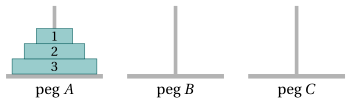
• Recursive idea. To move \(n\) disks from peg \(A\) to peg \(C\) using peg \(B\) as auxiliary peg:

  1. move the \(n-1\) smallest disks from \(A\) to \(B\) (using \(C\) as auxiliary peg), recursively;

  2. move the largest disk \(n\) from \(A\) to \(C\);

  3. move the \(n-1\) smallest disks from \(B\) to \(C\) (using \(A\) as auxiliary peg), recursively.

• During steps 1 and 3, disk \(n\) is at the bottom of a peg and it is larger than all the moved disks, so it never violates the rules: the \(n-1\) disks can be moved as if disk \(n\) were not there.

Algorithm: Hanoi

Input: The number of disks \(n \ge 1\), the source peg \(from\), the destination peg \(to\), the auxiliary peg \(aux\)

Output: The sequence of moves that transfers disks \(1,2,\dots,n\) from \(from\) to \(to\)

1function Hanoi(n, from, to, aux)

2if \(n = 1\) then

3move disk \(1\) from \(from\) to \(to\)// base case

4else

5Hanoi\((n-1, from, aux, to)\)

6move disk \(n\) from \(from\) to \(to\)

7Hanoi\((n-1, aux, to, from)\)

8end

9end

Run in Colab:PythonC++Java

• The initial call is Hanoi\((n, A, C, B)\).

Observation 14.13: correctness of Hanoi

For every natural number \(n \ge 1\), if disks \(1, 2, \dots, n\) are the top \(n\) disks of peg \(from\) and all the disks on pegs \(to\) and \(aux\) are larger than \(n\), then Hanoi\((n, from, to, aux)\) moves disks \(1, 2, \dots, n\) on top of peg \(to\), respecting the rules.

Proof

We proceed by induction on \(n\).

• Base case (\(n = 1\)): the single move of disk \(1\) is valid, since disk \(1\) is the smallest disk.

• Inductive step (\(n \ge 2\)): by the inductive hypothesis, the call of line 5 correctly moves the tower of the \(n-1\) smallest disks from \(from\) to \(aux\) (disk \(n\) and the disks below it are larger, so they do not interfere). Then disk \(n\) is on top of peg \(from\), and every disk on peg \(to\) is larger than \(n\): line 6 moves disk \(n\) correctly. Finally, by the inductive hypothesis, the call of line 7 moves the \(n-1\) smallest disks from \(aux\) on top of disk \(n\).

□

Example 14.12: Tree of recursive calls of Hanoi(3, A, C, B)

Each node shows the call (with arguments \(n\), \(from\), \(to\), \(aux\)) and, in red, the move executed by the call itself (line 3 or line 6), numbered in the order of execution.

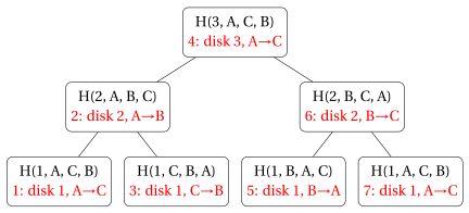
The moves are executed in the order of an in-order visit of the tree (left subtree, node, right subtree):

move	disk	from	to
1	1	A	C
2	2	A	B
3	1	C	B
4	3	A	C
5	1	B	A
6	2	B	C
7	1	A	C

The tree has \(7\) nodes and every node executes exactly one move: \(7\) moves in total.

14.8.1 Number of moves

• Let \(M(n)\) be the number of moves executed by Hanoi with \(n\) disks. From the pseudo-code,

  \[ M(n) = \begin{cases} 1 & \text{if } n = 1 \\ 2M(n-1) + 1 & \text{if } n \ge 2 \end{cases} \]

• Unrolling: \(M(n) = 2M(n-1) + 1 = 4M(n-2) + 2 + 1 = 8M(n-3) + 4 + 2 + 1 = \dots = 2^{n-1}M(1) + 2^{n-2} + \dots + 2 + 1 = 2^n - 1.\) We prove it formally:

Observation 14.14: number of moves of Hanoi

For every natural number \(n \ge 1\),

\[ M(n) = 2^n - 1. \]

Proof

We proceed by induction on \(n\).

• Base case (\(n = 1\)): \(M(1) = 1 = 2^1 - 1\).

• Inductive step (\(n \ge 2\)): assume \(M(n-1) = 2^{n-1} - 1\). Then

  \[ M(n) = 2M(n-1) + 1 = 2\big(2^{n-1} - 1\big) + 1 = 2^n - 2 + 1 = 2^n - 1. \]

□

• The number of steps satisfies \(S(1) = 2\) (lines 2–3) and \(S(n) = 2S(n-1) + 4\) for \(n \ge 2\) (lines 2, 5, 6, 7, plus the two recursive calls). Unrolling as above,

  \[ S(n) = 2^{n-1}S(1) + 4\big(2^{n-2} + \dots + 2 + 1\big) = 2^n + 4\big(2^{n-1} - 1\big) = 3 \cdot 2^n - 4 = \Theta(2^n), \]

  since \(\lim_{n\to\infty} (3\cdot 2^n - 4)/2^n = 3 \in \R_{>0}\).

• The depth of the recursion is only \(n\): the memory used by the call stack is \(\Theta(n)\).

14.8.2 Optimality

• The exponential number of moves is not a weakness of the algorithm: no algorithm can solve the problem with fewer moves.

Observation 14.15: optimality of Hanoi

Let \(M^*(n)\) be the minimum number of moves needed to transfer a tower of \(n \ge 1\) disks from one peg to another one. Then

\[ M^*(n) = 2^n - 1. \]

Proof (Sketch of proof)

Since the algorithm Hanoi uses \(2^n - 1\) moves, \(M^*(n) \le 2^n - 1\). We show \(M^*(n) \ge 2^n - 1\) by induction on \(n\). For \(n=1\), at least one move is needed.

Let \(n \ge 2\). The largest disk \(n\) must be moved at least once. Consider its first move, from the source peg to some other peg \(P\): at that moment disk \(n\) is the only disk on the source peg and peg \(P\) is empty, so the \(n-1\) smaller disks are all stacked on the third peg. Moving them there from the source peg required at least \(M^*(n-1)\) moves.

Consider now the last move of disk \(n\), onto the destination peg. After this move, the \(n-1\) smaller disks are all stacked on a peg different from the destination, and they must still be transferred on top of disk \(n\): this requires at least \(M^*(n-1)\) further moves.

These two groups of moves are distinct (one happens before the first move of disk \(n\), the other after its last move), hence

\[ M^*(n) \ge M^*(n-1) + 1 + M^*(n-1) = 2M^*(n-1) + 1 \ge 2\big(2^{n-1}-1\big) + 1 = 2^n - 1. \]

□

The Hanoi algorithm executes \(M(n) = 2^n - 1\) moves and \(S(n) = 3 \cdot 2^n - 4 = \Theta(2^n)\) steps, with depth of recursion \(n\). The number of moves is optimal: every algorithm must output \(2^n - 1\) moves, so the running time of any algorithm for this problem is exponential in \(n\) (and therefore doubly exponential in the input size \(|I| = \Theta(\log_2 n)\)).

• With \(n = 64\) disks (the original legend) and one move per second, \(2^{64} - 1\) seconds are more than \(5.8 \cdot 10^{11}\) years.

14.9 Summary

algorithm	recurrence for \(S(n)\)	\(S(n)\)	calls	depth
Factorial	\(S(n) = S(n-1) + 2\)	\(2n+2 = \Theta(n)\)	\(n+1\)	\(n+1\)
Fib (naive)	\(S(n) = S(n-1) + S(n-2) + 2\)	\(4F(n+1)-2 = 2^{\Theta(n)}\)	\(2F(n+1)-1\)	\(\max(n,1)\)
RecursiveGCD	\(m_{k+2} < m_k/2\) (Obs. [Observation 14.11](#box-19-obsGCDHalving))	\(O(\log_2 m)\)	\(\le 2\lfloor \log_2 m\rfloor + 3\)	= calls
FastPower	\(S(n) = S(\lfloor n/2 \rfloor) + 4\)	\(4\lfloor \log_2 n\rfloor + 6 = \Theta(\log_2 n)\)	\(\lfloor \log_2 n\rfloor + 2\)	= calls
Hanoi	\(S(n) = 2S(n-1) + 4\)	\(3\cdot 2^n - 4 = \Theta(2^n)\)	\(2^n - 1\)	\(n\)

• A recursive algorithm solves the base cases directly and reduces every other instance to strictly smaller instances of the same problem; this guarantees termination.

• The execution is described by the tree of recursive calls: the number of steps depends on the number of nodes, the memory used by the call stack on the depth of the tree.

• Correctness is proved by (strong) induction on the size of the input: base cases \(\leftrightarrow\) base of the induction, recursive step \(\leftrightarrow\) inductive step (as initialization and maintenance for loop invariants).

• The number of steps is described by a recurrence for \(S(n)\): decreasing by one with constant work gives \(\Theta(n)\) (Factorial); halving with constant work gives \(\Theta(\log_2 n)\) (FastPower); two calls on \(n-1\) give \(\Theta(2^n)\) (Hanoi).

• Recursion can be very inefficient when the same subproblems are solved many times (naive Fib): this motivates Dynamic Programming.

• A tail-recursive algorithm (RecursiveGCD) can be directly rewritten as a loop.

---

Exercises on this chapter: Recursion

Interactive lab

The algorithm of the chapter, one step at a time: move the sliders and press ▶. The same graph full page, with the other ones of the course, is in the interactive lab.