6.14 Piecewise linear functions

Technique: continuous with piece binaries · Script: python/cap03_links.py · All the techniques

The link in words

The cost is not proportional to the quantity: it changes in brackets — discounts above a threshold, surcharges beyond a capacity, banded tariffs. The function \(g(q)\) is continuous and piecewise linear, with breakpoints \(q_0 < q_1 < \dots < q_p\) and values \(g_0, \dots, g_p\).

The constraints

With \(\lambda_k \ge 0\) the weights of the convex combination and \(w_t \in \{0,1\}\) the indicator of piece \(t\) (between \(q_{t-1}\) and \(q_t\)):

\[ \begin{aligned} \sum_{k=0}^{p} \lambda_k &= 1 &&\qquad (1 \text{ constraint}),\\ q &= \sum_{k=0}^{p} q_k \lambda_k &&\qquad (1 \text{ constraint}),\\ g(q) &= \sum_{k=0}^{p} g_k \lambda_k &&\qquad (1 \text{ constraint}),\\ \sum_{t=1}^{p} w_t &= 1 &&\qquad (1 \text{ constraint}),\\ \lambda_k &\le \!\!\sum_{t \,:\, k \in \{t-1,\,t\}}\!\! w_t, \quad \forall k &&\qquad (p + 1 \text{ constraints}). \end{aligned} \]

The proof

The last group is adjacency: \(\lambda_k\) can be positive only if the chosen piece has \(q_k\) as an endpoint. Together with \(\sum_t w_t = 1\) the piece is unique, so at most two consecutive \(\lambda\) are positive, and then \((q, g(q))\) is a point of the segment between \((q_{t-1}, g_{t-1})\) and \((q_t, g_t)\): that is, a point of the graph. Without adjacency one could mix non-consecutive nodes, and \((q, g)\) would land in the lower convex envelope of the graph — below the function.

If the function is convex adjacency is superfluous, otherwise it is not

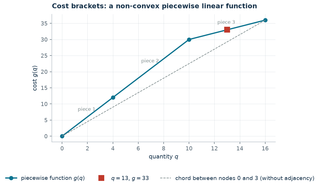
When \(g\) is convex and one minimises, the lower convex envelope coincides with the function and the optimal \(\lambda\) turn out adjacent automatically: the model without binaries is already correct. When \(g\) is not convex — the case of quantity discounts, where marginal cost falls — the difference shows immediately. With breakpoints \((0, 4, 10, 16)\), values \((0, 12, 30, 36)\) and demand \(q \ge 13\):

Formulation	optimal value
without adjacency (free convex combination)	\(117/4 = 29.25\)
with adjacency	\(33\)

The first mixes nodes \(0\) and \(3\) (the only nonzero \(\lambda\)) and returns a cost the function attains nowhere: it is the value of the envelope, not of the graph. The second mixes nodes \(2\) and \(3\), adjacent, and gives the exact value \(g(13) = 30 + 6 \cdot \tfrac{3}{6} = 33\).

Cost brackets

The strength of the relaxation

Two things must not be confused: adjacency changes the integer set (the two models have different optima, \(29.25\) and \(33\)), but not the strength of the relaxation — with \(w_t\) fractional the adjacency constraint does not bite and the two models share the same \(z(\mathit{LP}^+) = 117/4\).

In gurobipy

m.addConstr(lam.sum() == 1, name="convex")
m.addConstr(q == gp.quicksum(nodes[k] * lam[k] for k in range(K + 1)), name="abscissa")
m.addConstr(w.sum() == 1, name="one_piece")
for k in range(K + 1):                       # adjacency: lambda_k only on the pieces touching k
    m.addConstr(lam[k] <= gp.quicksum(w[t] for t in (k - 1, k) if 0 <= t < K),
                name=f"adjacency{k}")

Gurobi also offers addGenConstrPWL and SOS2 types, which do the same job internally; here the manual formulation remains the main material, because it is the one whose correctness must be provable.