Production and workforce: two equivalent formulations
Class: MILP · Links: integer counts, workforce balance · Script: python/fam09_2_workforce.py
Difficulty: ★★★★★ · Time: 45–60 min

Problem 9.2
A shoe factory must plan its production over \(n \in \mathbb{Z}_{\ge 1}\) months. For every month \(t \in \{1, 2, \dots, n\}\), the value \(d_t \in \mathbb{Z}_{\ge 0}\) is the demand in pairs and \(p_t \in \mathbb{Q}_{>0}\) the cost of the raw materials for one pair. For every month \(t \in \{1, 2, \dots, n-1\}\), the value \(h_t \in \mathbb{Q}_{\ge 0}\) is the cost of keeping one pair in stock at the end of the month. At the start of the horizon the company has \(m_0 \in \mathbb{Z}_{\ge 0}\) workers; every worker works \(r \in \mathbb{Q}_{>0}\) hours a month and costs \(w \in \mathbb{Q}_{>0}\) euros a month, and producing one pair requires \(g \in \mathbb{Q}_{>0}\) labour hours. At the start of every month workers may be hired, at a cost of \(u \in \mathbb{Q}_{\ge 0}\) euros each; nobody is laid off. The company wants to decide how much to produce and how many workers to employ in every month, at minimum total cost.
The problem in words. We decide how much to produce, how much to keep in stock and how many workers to hire. The objective: minimum total cost (raw materials, storage, wages and hirings). The constraints: the demand must be met exactly; the production of a month cannot require more hours than the workers on duty can do.
Two formulations
The same decision can be written in two ways, and it is worth putting them side by side: it is the first case in the course where two apparently different models describe the same set of plans.
Formulation A: the hirings. The staffing variables are
integer and non-negative. A worker hired in month \(t\) stays until the end of the horizon, so he or she costs \(u\) once plus \(w\) for each of the remaining \(n - t + 1\) months. The wages of the \(m_0\) initial workers, \(m_0\, w\, n\), are a constant term: it is left out of the model and added to the final value.
Formulation B: the headcount. The staffing variables are
integer and non-negative, with \(y_t \ge y_{t-1}\) because nobody is laid off. The cost is \(w\, y_t\) every month, plus \(u\) for every hiring, that is \(u\,(y_n - m_0)\) in total, because the hirings are the increments of the headcount and the telescoping sum leaves only the endpoints.
Model
Variables. \(x_t \in \mathbb{Z}_{\ge 0}\) pairs produced in month \(t\); \(s_t \in \mathbb{Z}_{\ge 0}\) stock at the end of month \(t\) (for \(t \le n-1\)); \(y_t \in \mathbb{Z}_{\ge 0}\) workers on duty in month \(t\); \(z_t \in \mathbb{Z}_{\ge 0}\) workers hired at the start of month \(t\).
Model 9.2A — with the hirings.
Model 9.2B — with the headcount.
Description. The two formulations share the stock balances, one per month: what is produced plus what is in stock covers the demand exactly. The hours constraints, one per month, say that a month's production cannot require more hours than the workers on duty can do. Formulation \(B\) has in addition the initial headcount constraint, which starts from the \(m_0\) workers already employed, and the monotonicity constraints, one per month from the second on, which forbid layoffs. In \(A\) those same facts are hidden in the domain of the \(z_t\), which are non-negative.
The two formulations describe the same problem
The correspondence is
Feasibility. With this substitution the hours constraint of \(A\) becomes exactly that of \(B\); the conditions \(z_t \ge 0\) become \(y_t \ge y_{t-1}\), and \(y_1 \ge m_0\). The balances contain no staffing variables and stay identical: the correspondence is a bijection between the feasible plans of the two models.
Cost. The staffing cost in \(B\) equals
because \(z_j\) appears in every month from \(j\) onwards, that is \(n - j + 1\) times. The two objective functions differ by the constant \(m_0\, w\, n\) alone, and the two models have the same optima.
Why keep both
Formulation \(A\) has fewer constraints (no monotonicity) but cost coefficients that depend on the period; \(B\) has uniform coefficients and extends better if layoffs are added (a second family \(\ell_t \ge 0\) and the balance \(y_t = y_{t-1} + z_t - \ell_t\) suffice). On the instance the relaxations coincide as well: \(z(\mathit{LP}) = 15\,960\) for both. Two formulations equivalent over the integers are not always equivalent on the relaxation; here they are, and the check has to be made, not assumed.
The model in gurobipy
m = gp.Model("workforce_B")
x = m.addVars(n, vtype=GRB.INTEGER, name="x")
s = m.addVars(n - 1, vtype=GRB.INTEGER, name="s")
y = m.addVars(n, vtype=GRB.INTEGER, name="y")
m.setObjective(gp.quicksum(p[t] * x[t] for t in range(n))
               + gp.quicksum(h[t] * s[t] for t in range(n - 1))
               + gp.quicksum(w * y[t] for t in range(n)) + u * (y[n - 1] - m0), GRB.MINIMIZE)
m.addConstr(x[0] - s[0] == d[0], name="balance[0]")
m.addConstrs((x[t] + s[t - 1] - s[t] == d[t] for t in range(1, n - 1)), name="balance")
m.addConstr(x[n - 1] + s[n - 2] == d[n - 1], name=f"balance[{n - 1}]")
m.addConstrs((-g * x[t] + r * y[t] >= 0 for t in range(n)), name="hours")
m.addConstr(y[0] >= m0, name="initial_headcount")
m.addConstrs((-y[t - 1] + y[t] >= 0 for t in range(1, n)), name="no_layoffs")
The instance
\(n = 3\) months, \(m_0 = 2\) workers, \(w = 1500\), \(u = 100\), \(r = 160\) hours, \(g = 4\) hours per pair, \(h_t = 3\).
| \(t=1\) | \(t=2\) | \(t=3\) | |
|---|---|---|---|
| \(d_t\) | 60 | 100 | 140 |
| \(p_t\) | 15 | 15 | 15 |
With two workers the initial capacity is \(2 \cdot 160 / 4 = 80\) pairs a month: enough for the first month, not for the other two.
The model written on the data of the instance:
Constructive heuristic: the primal bound
Just-in-time production: every month one produces exactly the demand and hires the minimum number of workers needed. It is a constructive heuristic: a single solution is built, one element at a time, never backtracking.
- month 1: \(\lceil 4 \cdot 60/160 \rceil = 2\) workers, no hiring;
- month 2: \(\lceil 4 \cdot 100/160 \rceil = 3\) workers, one hiring;
- month 3: \(\lceil 4 \cdot 140/160 \rceil = 4\) workers, another hiring.
The cost, including the constant term \(m_0\, w\, n = 9000\), is \(z(\mathit{MILP}) \le \mathit{UB} = 18\,200\).
LP relaxation and dual: the dual bound
On formulation \(A\), with \(\mu_t\) free on each balance and \(\nu_t \ge 0\) on each hours constraint:
The same dual, written on the data of the instance:
Description. \(\mu_t\) is the value of one pair available in month \(t\) and \(\nu_t\) the price of one working hour. The objective prices the demand at those values and subtracts \(r\, m_0 \sum_t \nu_t\), that is, the hours the two initial workers supply for free. The first group of constraints are the columns of the \(x_t\): producing one pair is worth \(\mu_t\) and consumes \(g\) hours at price \(\nu_t\), and the balance cannot exceed the raw-material cost \(p_t\). The second are the columns of the \(s_t\): holding one pair in stock earns \(\mu_{t+1} - \mu_t\), which cannot exceed \(h_t\). The third are the columns of the \(z_j\): a worker hired in month \(j\) supplies \(r\) hours in each month from \(j\) onwards, and their value cannot exceed what that hire costs.
Recipe. \(\bar\nu_t = 0\): working hours are not priced, the hiring constraints are satisfied because the right-hand side is positive, and \(\mu_t \le p_t\) and \(\mu_{t+1} \le \mu_t + h_t\) remain. The largest feasible value is built forwards,
On the instance \(\bar\mu = (15, 15, 15)\) and \(\sum_t d_t\, \bar\mu_t = 15 \cdot 300 = 4500\), to which the constant term \(9000\) must be added:
It is the cost of the raw materials alone plus the wages of the workers already on duty: the extra workforce is given away.
Optimal solution
| \(t=1\) | \(t=2\) | \(t=3\) | |
|---|---|---|---|
| production \(x_t\) | 60 | 120 | 120 |
| headcount \(y_t\) | 2 | 3 | 3 |
| hirings \(z_t\) | 0 | 1 | 0 |
| stock \(s_t\) | 0 | 20 | — |
| \(UB\) | \(LB\) (dual) | \(z(\mathit{LP})\) | \(z(\mathit{LP}^+)\) | \(z(\mathit{MILP})\) | heuristic gap |
|---|---|---|---|---|---|
| 18200 | 13500 | 15960 | 15960 | 16660 | \(9.2\%\) |
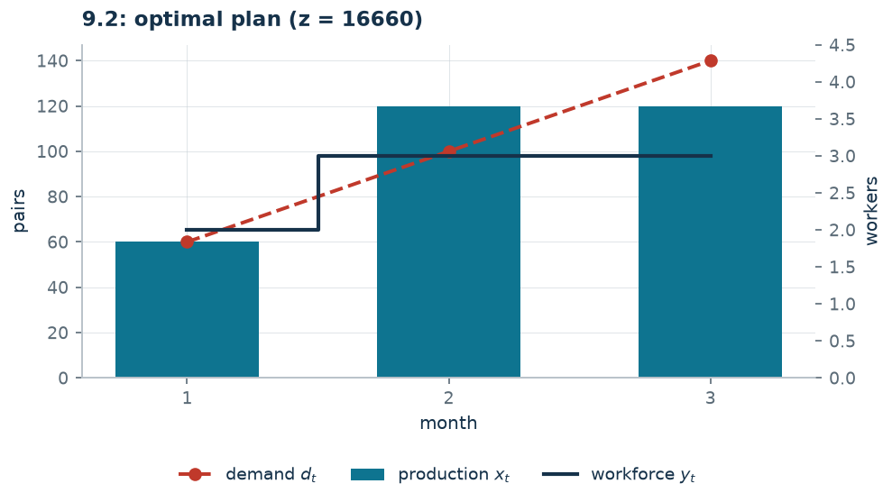
The optimal plan hires one worker instead of two and moves twenty pairs from the third month to the second: paying \(3\) euros of storage for twenty pairs costs \(60\) euros against the \(1600\) of a hiring in the third month.
Additional considerations
- The monotonicity constraint is what makes the problem non-trivial: if one could lay off at no cost, every month would pick on its own the smallest staff able to produce \(x_t\), and that family would disappear. The problem would not split into \(n\) independent problems, though: the stocks \(s_t\) still tie each month to the next.
- The variables \(x_t\) and \(s_t\) are declared integer because pairs of shoes do not split. Here they could be left continuous without changing the optimum --- but not because the matrix is totally unimodular: it is not, as the relaxation shows, worth \(15\,960\) against an integer optimum of \(16\,660\). The reason is more local: once the staff \(y\) is fixed at integer values, what is left in \((x, s)\) is a balance problem with an interval matrix, totally unimodular, and integer right-hand sides (the demands, and the capacities \(r\, y_t / g = 40\, y_t\)); an optimal vertex of it is therefore integer. It is an argument about the subproblem, not about the whole model.
- The constant term \(m_0\, w\, n\) must be remembered in every comparison: forgetting it makes formulation \(A\) look far cheaper than \(B\).
Additional modelling questions
9.2.1 — Overtime
Every worker may do up to \(40\) hours of overtime a month, paid \(25\) euros an hour. How does the model change? Is it worth using them?
A worked variant: very expensive hirings
The hiring cost goes up from \(100\) to \(3000\) euros (selection and training).
Only the datum \(u\) changes. The new optimum is \(19\,560\), that is \(2900\) euros more. The plan does not change: one worker is hired anyway, because without that hiring the problem is infeasible (\(4 \cdot 120 / 160 = 3\) workers are needed in any case). The difference is exactly \(3000 - 100 = 2900\): the extra cost of an unavoidable hiring. It is a useful example of sensitivity analysis carried out by re-solving the model.
The variant adds no constraint: it changes a datum, \(u = 3000\) instead of \(100\). Model, dual and recipe are those of the base problem, and the certificate does not notice the change, because \(\mu_t\) is the lowest cost of having a pair available in month \(t\) and the hiring cost does not appear there: the bound stays \(13500\), while the optimum rises from \(16660\) to \(19560\). It is the limiting case of this chapter: a correct dual bound can be completely insensitive to the datum that moves the problem, and here it is the heuristic that follows it.
| value | what it is | |
|---|---|---|
| \(\mathit{UB}\) | \(24000\) | heuristic solution |
| \(\mathit{LB}\) | \(13500\) | dual certificate built by hand |
| \(z(\mathit{LP})\) | \(17490\) | relaxation without the bounds |
| \(z(\mathit{LP}^+)\) | \(17490\) | relaxation with the bounds |
| \(z(\mathit{MILP})\) | \(19560\) | optimum of the MILP |
Code
Complete script —
python/fam09_2_workforce.py
(reproducible with python3 python/fam09_2_workforce.py from the python/
folder). Notebook —
notebooks/fam09_2_workforce.ipynb
— which opens in Colab from the badge at the top of the page.
Show the complete script — python/fam09_2_workforce.py (275 lines)
"""Problem 9.2 -- Production and workforce: two equivalent formulations.

The same decision written twice: with the *hirings* z_t (formulation A) or with
the *workforce* y_t (formulation B). We prove that they have the same set of
feasible plans and the same optimum, and we compare the relaxations. This is the
theme of chapter 4: two formulations may be compared only after proving that they
describe the same integer set.
"""
import gurobipy as gp
import pandas as pd
from gurobipy import GRB

from mip import (ammissibile, dualita_forte, due_rilassamenti, frazione, nuovo_modello,
                 rilassamenti,
                 registra_bound, rilassamenti, rilassamento, risolvi, valuta)
from stile import ARANCIO, BLU, ROSSO, TEAL, intestazione, plt, salva_dati, salva_figura
from esteso import salva_modello

R = range

# ---------- 1. MODEL AND INSTANCE ----------
intestazione("9.2 Production and workforce: hirings (A) or workforce (B)")
d2 = [60, 100, 140]        # demand of the three months (pairs)
p2 = [15, 15, 15]          # production cost per pair
h2 = [3, 3]                # storage cost at the end of the month
w2, r2, g2, u2, m2, r0 = 1500, 160, 4, 100, 2, 0
n2 = len(d2)
salva_dati(pd.DataFrame({"month": R(1, n2 + 1), "demand": d2, "cost_pair": p2}), "fam09_2_dati")
print(f"  {m2} workers at the start, {r2} h a month each, {g2} h per pair: the initial")
print(f"  capacity is {m2 * r2 // g2} pairs a month. Wage {w2}, hiring {u2}.")


def modello_A(d, p, h, w, r, g, u, m0, r0):
    """Formulation A: z_t = how many workers are hired at the start of month t."""
    n = len(d)
    mm = nuovo_modello("workforce_A")
    x = mm.addVars(n, vtype=GRB.INTEGER, name="x")
    s = mm.addVars(n - 1, vtype=GRB.INTEGER, name="s")
    z = mm.addVars(n, vtype=GRB.INTEGER, name="z")
    mm.setObjective(gp.quicksum(p[t] * x[t] for t in R(n))
                    + gp.quicksum(h[t] * s[t] for t in R(n - 1))
                    + gp.quicksum((u + w * (n - t)) * z[t] for t in R(n)), GRB.MINIMIZE)
    mm.addConstr(x[0] - s[0] == d[0] - r0, name="balance[0]")
    mm.addConstrs((x[t] + s[t - 1] - s[t] == d[t] for t in R(1, n - 1)), name="balance")
    mm.addConstr(x[n - 1] + s[n - 2] == d[n - 1], name=f"balance[{n - 1}]")
    mm.addConstrs((-g * x[t] + gp.quicksum(r * z[j] for j in R(t + 1)) >= -r * m0
                   for t in R(n)), name="hours")
    return mm, x, s, z


def modello_B(d, p, h, w, r, g, u, m0, r0):
    """Formulation B: y_t = how many workers are employed in month t (workforce)."""
    n = len(d)
    mm = nuovo_modello("workforce_B")
    x = mm.addVars(n, vtype=GRB.INTEGER, name="x")
    s = mm.addVars(n - 1, vtype=GRB.INTEGER, name="s")
    y = mm.addVars(n, vtype=GRB.INTEGER, name="y")
    # the workforce pays the wage every month; the hirings are the increments y_t - y_{t-1}
    mm.setObjective(gp.quicksum(p[t] * x[t] for t in R(n))
                    + gp.quicksum(h[t] * s[t] for t in R(n - 1))
                    + gp.quicksum(w * y[t] for t in R(n))
                    + u * (y[n - 1] - m0), GRB.MINIMIZE)   # total hirings = y_n - m0
    mm.addConstr(x[0] - s[0] == d[0] - r0, name="balance[0]")
    mm.addConstrs((x[t] + s[t - 1] - s[t] == d[t] for t in R(1, n - 1)), name="balance")
    mm.addConstr(x[n - 1] + s[n - 2] == d[n - 1], name=f"balance[{n - 1}]")
    mm.addConstrs((-g * x[t] + r * y[t] >= 0 for t in R(n)), name="hours")
    mm.addConstr(y[0] >= m0, name="initial_workforce")
    mm.addConstrs((-y[t - 1] + y[t] >= 0 for t in R(1, n)), name="no_layoffs")
    return mm, x, s, y


def duale_A(d, p, h, w, r, g, u, m0, r0):
    """max sum_t b_t mu_t - r m0 sum_t nu_t;  mu_t - g nu_t <= p_t;
    -mu_t + mu_{t+1} <= h_t;  r sum_{t >= j} nu_t <= u + w (n - j);  mu free, nu >= 0."""
    n = len(d)
    b = [d[0] - r0] + d[1:n - 1] + [d[n - 1]]
    dl = nuovo_modello("dual_workforce")
    mu = dl.addVars(n, lb=-GRB.INFINITY, name="mu")
    nu = dl.addVars(n, name="nu")
    dl.setObjective(gp.quicksum(b[t] * mu[t] for t in R(n))
                    - r * m0 * gp.quicksum(nu[t] for t in R(n)), GRB.MAXIMIZE)
    dl.addConstrs((mu[t] - g * nu[t] <= p[t] for t in R(n)), name="rc_x")
    dl.addConstrs((-mu[t] + mu[t + 1] <= h[t] for t in R(n - 1)), name="rc_s")
    dl.addConstrs((r * gp.quicksum(nu[t] for t in R(j, n)) <= u + w * (n - j) for j in R(n)),
                  name="rc_z")
    return dl


mA, xA, sA, zA = modello_A(d2, p2, h2, w2, r2, g2, u2, m2, r0)
salva_modello(mA, "fam09_2_primale")
mB, xB, sB, yB = modello_B(d2, p2, h2, w2, r2, g2, u2, m2, r0)
salva_modello(mB, "fam09_2_primale_b")
costante_A = m2 * w2 * n2          # the wage of the initial workers, outside model A
zA_val = risolvi(mA) + costante_A
zB_val = risolvi(mB)
print(f"  Formulation A (hirings):   z = {frazione(zA_val)} "
      f"(of which {costante_A} of wages of the initial workers, a constant term)")
print(f"  Formulation B (workforce): z = {frazione(zB_val)}")
assert abs(zA_val - zB_val) < 1e-6, (zA_val, zB_val)
print("  The two optima coincide: the two formulations describe the same problem.")
print("  Plan A: production " + ", ".join(frazione(xA[t].X) for t in R(n2))
      + "; hirings " + ", ".join(frazione(zA[t].X) for t in R(n2)))
print("  Plan B: production " + ", ".join(frazione(xB[t].X) for t in R(n2))
      + "; workforce " + ", ".join(frazione(yB[t].X) for t in R(n2)))

# ---------- 2. THE LP RELAXATION ----------
zlp2, zlp2r, _ = rilassamenti(mA)

# ---------- 3. THE DUAL OF THE RELAXATION (LOWER BOUND) ----------
dl2 = duale_A(d2, p2, h2, w2, r2, g2, u2, m2, r0)
salva_modello(dl2, "fam09_2_duale")
# recipe: nu = 0 (the hours are not charged) and mu_t = cheapest way to have a pair
# available in month t
mu = []
for t in R(n2):
    mu.append(p2[t] if t == 0 else min(mu[t - 1] + h2[t - 1], p2[t]))
mano = {f"mu[{t}]": mu[t] for t in R(n2)}
lb2_var, viol = valuta(dl2, mano)
assert viol <= 1e-9, viol
lb2 = lb2_var + costante_A
print("  Hand-built dual: nu = 0 (working hours are not charged) and")
print("  mu_t = min(mu_{t-1} + h, p_t)")
print(f"    mu = " + ", ".join(frazione(v) for v in mu)
      + f"  ->  lb = {frazione(lb2_var)} + {costante_A} = {frazione(lb2)}")
dualita_forte(dl2, zlp2)
zlp2, zlp2r = zlp2 + costante_A, zlp2r + costante_A

# ---------- 4. CONSTRUCTIVE HEURISTIC (UPPER BOUND) ----------
intestazione("9.2 Heuristic, dual and bounds")
# constructive heuristic: produce the demand of the month, and hire only when the hours are not enough
organico, assunzioni, prod = m2, [0] * n2, []
for t in R(n2):
    prod.append(d2[t])
    servono = -(-g2 * d2[t] // r2)               # ceil
    if organico < servono:
        assunzioni[t] = servono - organico
        organico = servono
    print(f"  Month {t + 1}: {d2[t]} pairs are produced, "
          f"ceil({g2} * {d2[t]} / {r2}) = {servono} workers are needed; workforce "
          f"{organico - assunzioni[t]} -> {assunzioni[t]} are hired")
ub2 = sum(p2[t] * prod[t] for t in R(n2)) \
    + sum(assunzioni[t] * (u2 + w2 * (n2 - t)) for t in R(n2)) + costante_A
sol_eur = {f"x[{t}]": prod[t] for t in R(n2)} | {f"z[{t}]": assunzioni[t] for t in R(n2)} \
    | {f"s[{t}]": 0 for t in R(n2 - 1)}
assert ammissibile(mA, sol_eur)
print(f"  Cost of the heuristic: ub = {frazione(ub2)}")
riga = registra_bound("2 workforce", ub2, lb2, zlp2, zlp2r, zA_val)
salva_dati(pd.DataFrame([riga]), "fam09_2_bound")
assert lb2 <= zlp2 <= zA_val <= ub2 + 1e-9

# ---------- 5. THE EQUIVALENCE, VERIFIED ----------
intestazione("9.2 The equivalence between the two formulations, verified")
print("  The correspondence is y_t = m0 + sum_{j <= t} z_j, that is z_t = y_t - y_{t-1}")
print("  (with y_0 = m0). On the optimal plans:")
yA = [m2 + sum(round(zA[j].X) for j in R(t + 1)) for t in R(n2)]
print("    from A: implied workforce = " + ", ".join(str(v) for v in yA))
print("    from B: workforce         = " + ", ".join(str(round(yB[t].X)) for t in R(n2)))
zB_implicite = [round(yB[0].X) - m2] + [round(yB[t].X) - round(yB[t - 1].X) for t in R(1, n2)]
print("    from B: implied hirings   = " + ", ".join(str(v) for v in zB_implicite))
assert sum(v * (u2 + w2 * (n2 - t)) for t, v in enumerate(zB_implicite)) + costante_A \
    == sum(round(zA[t].X) * (u2 + w2 * (n2 - t)) for t in R(n2)) + costante_A
print("  The staff cost is the same: A charges every hiring once for all the months that")
print("  remain, B charges the workforce month by month. Same total, counted two ways.")

# ---------- 6. COMPARING THE RELAXATIONS OF THE TWO FORMULATIONS ----------
zlpA, _, _ = rilassamento(mA, rafforzato=True)
zlpB, _, _ = rilassamento(mB, rafforzato=True)
print(f"  Relaxations: A -> {frazione(zlpA + costante_A)}   B -> {frazione(zlpB)}   "
      f"z(MILP) = {frazione(zA_val)}")
salva_dati(pd.DataFrame([{"formulation": "A (hirings)", "z_lp": zlpA + costante_A,
                          "z_milp": zA_val},
                         {"formulation": "B (workforce)", "z_lp": zlpB, "z_milp": zB_val}]),
           "fam09_2_formulazioni")

# ---------- 7. ADDITIONAL MODELLING QUESTIONS ----------
varianti = {}


def variante(nome, m, costante=0.0):
    z = risolvi(m) + costante
    print(f"  {nome:70s} z = {frazione(z)}")
    return z


# 2a: hiring costs much more (3000 instead of 100)
m, x, s, y = modello_B(d2, p2, h2, w2, r2, g2, 3000, m2, r0)
varianti["2a"] = variante("2a. A hiring costs 3000 euros instead of 100", m)
print("     workforce: " + ", ".join(str(round(y[t].X)) for t in R(n2))
      + ";  production: " + ", ".join(str(round(x[t].X)) for t in R(n2)))
# 2b: overtime, up to 40 extra hours per worker a month, at 25 euros an hour
m, x, s, y = modello_B(d2, p2, h2, w2, r2, g2, u2, m2, r0)
o = m.addVars(n2, name="o")
m.update()
for t in R(n2):
    m.chgCoeff(m.getConstrByName(f"hours[{t}]"), o[t], 1.0)   # the available hours grow
m.addConstrs((o[t] <= 40 * y[t] for t in R(n2)), name="max_overtime")
m.setObjective(m.getObjective() + gp.quicksum(25 * o[t] for t in R(n2)), GRB.MINIMIZE)
varianti["2b"] = variante("2b. Overtime: up to 40 h per worker, 25 euros an hour", m)
print("     overtime used: " + ", ".join(frazione(o[t].X) for t in R(n2))
      + "  (none: producing early and storing costs less)")
salva_dati(pd.DataFrame({"variant": list(varianti), "z": list(varianti.values())}),
           "fam09_2_varianti")

# ---------- 8. THE SANDWICH ON THE VARIANT 2a ----------
intestazione("9.2a The sandwich on the variant: hiring costs 3000 euros")
U2A = 3000

# The variant adds no constraint: it changes a datum. Model and dual are the
# same, with u = 3000, and the dual recipe is the same too --- what changes is
# the value it returns, and that is exactly the point: the certificate follows
# the data without the model being touched.
m2a, x2a, s2a, z2a = modello_A(d2, p2, h2, w2, r2, g2, U2A, m2, r0)
salva_modello(m2a, "fam09_2a_primale")
d2a_ = duale_A(d2, p2, h2, w2, r2, g2, U2A, m2, r0)
salva_modello(d2a_, "fam09_2a_duale")

# -- feasible heuristic: the same rule, with the new hiring cost --
print("Constructive heuristic: one produces the demand of the month and hires only when the")
print("hours of the workers on duty are not enough. The rule does not change; its cost does.")
operai = m2
assunti = [0] * n2
for tt in R(n2):
    servono = -(-g2 * d2[tt] // r2)                      # arrotondamento per eccesso
    if servono > operai:
        assunti[tt] = servono - operai
        operai = servono
        print(f"  month {tt + 1}: {servono} workers are needed, {assunti[tt]} hired")
    else:
        print(f"  month {tt + 1}: the {operai} workers on duty are enough")
ub2a = (sum(p2[tt] * d2[tt] for tt in R(n2))
        + sum((U2A + w2 * (n2 - tt)) * assunti[tt] for tt in R(n2)) + costante_A)
sol_2a = ({f"x[{tt}]": d2[tt] for tt in R(n2)} | {f"s[{tt}]": 0 for tt in R(n2 - 1)}
          | {f"z[{tt}]": assunti[tt] for tt in R(n2)})
assert ammissibile(m2a, sol_2a), "the heuristic solution of the variant must be feasible"
print(f"  ub = {frazione(ub2a)}")

# -- dual certificate: the recipe of the base problem, on the new data --
mu_2a = []
for tt in R(n2):
    tetto = p2[tt]
    mu_2a.append(tetto if tt == 0 else min(mu_2a[tt - 1] + h2[tt - 1], tetto))
mano_2a = {f"mu[{tt}]": mu_2a[tt] for tt in R(n2)}
lb2a_var, viol_2a = valuta(d2a_, mano_2a)
assert viol_2a <= 1e-9, viol_2a
lb2a = lb2a_var + costante_A                 # as in the base problem: the wages of the
                                             # initial workers sit outside formulation A
print("Dual solution by hand: nu = 0 (the hours are given away) and mu_t = the lowest cost to")
print("  have a pair available in month t, that is min(mu_{t-1} + h_{t-1}, p_t), as in the")
print(f"  base problem: mu = {[frazione(v) for v in mu_2a]}")
print(f"  ->  lb = {frazione(lb2a_var)} + {costante_A} = {frazione(lb2a)}")
zlp2a, zlp2ar, _ = due_rilassamenti(m2a, d2a_)
zlp2a, zlp2ar = zlp2a + costante_A, zlp2ar + costante_A
z2a_val = risolvi(m2a) + costante_A
riga_2a = registra_bound("2a hiring at 3000", ub2a, lb2a, zlp2a, zlp2ar, z2a_val)
salva_dati(pd.DataFrame([riga_2a]), "fam09_2a_bound")
assert lb2a <= zlp2a <= z2a_val <= ub2a + 1e-9

# ---------- 9. FIGURE ----------
fig, ax = plt.subplots(figsize=(7.0, 3.2))
mesi = list(R(1, n2 + 1))
ax.bar(mesi, [xB[t].X for t in R(n2)], color=TEAL, width=0.55, label="production $x_t$")
ax.plot(mesi, d2, "o--", color=ROSSO, label="demand $d_t$")
ax2 = ax.twinx()
ax2.step(mesi, [yB[t].X for t in R(n2)], where="mid", color=BLU, lw=2, label="workforce $y_t$")
ax2.set_ylabel("workers", color=BLU)
ax2.set_ylim(0, max(yB[t].X for t in R(n2)) + 1.5)
ax2.grid(False)
ax.set_xticks(mesi)
ax.set_xlabel("month")
ax.set_ylabel("pairs")
ax.set_title(f"9.2: optimal plan (z = {frazione(zB_val)})")
ax.legend(fontsize=8, loc="upper left")
ax2.legend(fontsize=8, loc="lower right")
salva_figura(fig, "cap09_manodopera_ottimo")
print("Done.")