Lot sizing with a fixed setup cost
Class: MILP · Links: fixed cost (big-M read off the data) · Script: python/fam09_1_lotsizing.py
Difficulty: ★★★★☆ · Time: 45–60 min

Problem 9.1
A company has to plan the production of a single product over \(n \in \mathbb{Z}_{\ge 1}\) periods. For every period \(t\), \(d_t\) is the demand, \(p_t\) the cost of producing one unit and \(q_t\) the fixed cost to be paid if production is set up in that period. For every \(t \le n-1\), \(h_t\) is the cost of keeping one unit in the warehouse at the end of the period. The initial stock is \(r_0\), the required final stock is \(r_n\). All the demand must be met at minimum total cost.
The problem in words. We decide how much to produce in each period, and consequently how much is left in the warehouse. The objective: minimum total cost (production, setups and warehouse). The constraints: the demand of every period must be met exactly, and one cannot produce without paying the fixed cost. This is the lot sizing problem with setup.
Model
Variables. \(x_t \ge 0\) units produced, \(s_t \ge 0\) stock at the end of period \(t\) (\(t \le n-1\)), \(y_t \in \{0,1\}\) production setup.
The link. The constraint \(x_t \le M_t\, y_t\) says: if \(y_t = 0\) then \(x_t = 0\) (no production without a setup); if \(y_t = 1\) the constraint is not restrictive. The opposite direction — if \(x_t = 0\) then \(y_t = 0\) — is imposed by no constraint but follows from optimality, because setting \(y_t = 0\) stays feasible and saves \(q_t\). If \(q_t > 0\) every optimal solution has \(y_t = 0\); if \(q_t = 0\) the saving is nil and one can only say that an optimal solution with \(y_t = 0\) exists.
The big-M is read off the data
A valid \(M_t\) must be at least the largest quantity it is worth producing in period \(t\). In an optimal solution one never produces more than the demand that is left to cover:
In the first period the initial inventory, which is a datum, can be subtracted: \(M_1 = \sum_{\tau = 1}^{n} d_\tau + r_n - r_0\). From the second period on the incoming inventory is not known in advance, and the bound stays the one above. On the instance \(r_0 = 0\), so the two values coincide.
Any larger value is still valid but weakens the LP relaxation; any smaller value may cut off optimal solutions. On the instance \(M = (110, 90, 80, 50, 10)\): the big-M of the last period is \(10\), not \(110\).
The model in gurobipy
m = gp.Model("lotsizing")
x = m.addVars(n, name="x")
s = m.addVars(n - 1, name="s")
y = m.addVars(n, vtype=GRB.BINARY, name="y")
m.setObjective(gp.quicksum(p[t] * x[t] for t in range(n))
               + gp.quicksum(q[t] * y[t] for t in range(n))
               + gp.quicksum(h[t] * s[t] for t in range(n - 1)), GRB.MINIMIZE)
m.addConstr(x[0] - s[0] == d[0] - r0, name="balance[0]")
m.addConstrs((x[t] + s[t - 1] - s[t] == d[t] for t in range(1, n - 1)), name="balance")
m.addConstr(x[n - 1] + s[n - 2] == d[n - 1] + rn, name=f"balance[{n - 1}]")
m.addConstrs((-x[t] + M[t] * y[t] >= 0 for t in range(n)), name="setup")
The instance
\(n = 5\) days, \(r_0 = r_n = 0\), total demand \(110\) units.
| \(t=1\) | \(t=2\) | \(t=3\) | \(t=4\) | \(t=5\) | |
|---|---|---|---|---|---|
| \(d_t\) | 20 | 10 | 30 | 40 | 10 |
| \(p_t\) | 2 | 3 | 2 | 3 | 2 |
| \(q_t\) | 50 | 50 | 50 | 50 | 50 |
| \(M_t\) | 110 | 90 | 80 | 50 | 10 |
| \(h_t\) | 1 | 1 | 1 | 1 | — |
The model written on the data of the instance:
Constructive heuristics: the primal bound
(a) Lot-for-lot. One produces every day exactly the demand: no stock, but a setup every day. Cost \(270 + 250 = 520\).
(b) Least unit cost. One starts from the first uncovered period and covers with a single set-up the number of periods that minimises the average cost per unit,
then starts again. Cost \(O(n^2)\). The numerator holds only the set-up and the inventory: the production cost \(p\) does not appear, because the alternatives being compared all start in the same period and cover the same demands anyway, so they pay the same \(p\) per unit and it does not change the comparison. The numbers below are therefore incremental costs of set-up plus inventory, not the full cost of one unit.
- period 1: covers up to 2, quantity \(30\), average cost \(2\);
- period 3: covers up to 4, quantity \(70\), average cost \(\approx 1.286\);
- period 5: covers only itself, quantity \(10\), average cost \(5\).
Setups on days \(1, 3, 5\), for a cost of \(420\). Keeping the better of the two, \(z(\mathit{MILP}) \le \mathit{UB} = 420\).
LP relaxation and dual: the dual bound
With \(\mu_t\) free on every balance and \(\pi_t \ge 0\) on every setup constraint:
The same dual, written on the data of the instance:
The recipe. \(\bar\pi_t = 0\): the setups are given away. What is left is \(\mu_t \le p_t\) and \(\mu_{t+1} \le \mu_t + h_t\), and the largest feasible value is built forward,
The reading is direct: \(\bar\mu_t\) is the lowest unit cost of having one unit available in period \(t\), either by producing it then, or by producing it earlier and keeping it in the warehouse. On the instance \(\bar\mu = (2, 3, 2, 3, 2)\) and
It is the production cost if the setups were free: valid, and deliberately optimistic.
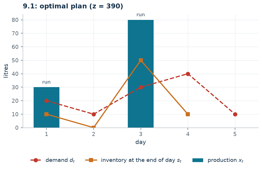
What the solver says. \(z(\mathit{LP}) = z(\mathit{LP}^+) = 3890/11 \approx 353.6\): the relaxation does pay for the setups, in fractions (\(\pi_t = q_t/M_t\) is feasible). The integer optimum sets up on days 1 and 3.
| \(t=1\) | \(t=2\) | \(t=3\) | \(t=4\) | \(t=5\) | |
|---|---|---|---|---|---|
| setup \(y_t\) | 1 | 0 | 1 | 0 | 0 |
| production \(x_t\) | 30 | 0 | 80 | 0 | 0 |
| stock \(s_t\) | 10 | 0 | 50 | 10 | — |
| \(UB\) | \(LB\) (dual) | \(z(\mathit{LP})\) | \(z(\mathit{LP}^+)\) | \(z(\mathit{MILP})\) | heuristic gap |
|---|---|---|---|---|---|
| 420 | 270 | \(3890/11\) | \(3890/11\) | 390 | \(7.7\%\) |
Additional considerations
- The problem is solved in \(O(n^2)\) time by the Wagner–Whitin dynamic program. Least unit cost is not that algorithm: it is a myopic rule that looks at one setup at a time, and indeed it stops at \(420\) against \(390\).
- The valid inequality \(x_t \le M_t\) adds nothing: \(M_t\) is already the largest useful production, and indeed \(z(\mathit{LP}) = z(\mathit{LP}^+)\).
- An alternative formulation with variables \(x_{t\tau}\) (``produced in \(t\), sold in \(\tau\)'') has an integral relaxation but \(O(n^2)\) variables: the typical trade-off between the size of the model and the quality of the relaxation.
Additional modelling questions
9.1.1 — Minimum lot
If production takes place on a day, at least \(25\) units must be produced. How does the model change? What is the new optimum?
A worked variant: daily capacity
The plant cannot produce more than \(35\) units a day.
One adds the \(n\) linear constraints
Alternatively one can replace the big-M with \(M_t' = \min(M_t, 35)\): constraint then acts both as the activation link and as the capacity constraint, exactly as in the capacitated facility location of chapter ``Location and covering''. On the instance the optimal plan with only two runs is no longer feasible (\(80 > 35\)) and the optimum rises to \(470\).
The cap \(x_t \le 35\) adds to the dual a family \(\nu_t \ge 0\) with right-hand side \(-35\): it enters the objective with a negative sign and loosens the column of \(x_t\). Raising \(\nu_t\) by one unit lifts the cap on \(\mu_t\) and collects \(d_t\), but costs \(35\), so it only pays where the demand exceeds the capacity; and on this instance not even the busiest day justifies it, because the chain of the stocks already keeps \(\mu_t\) below the cap. The certificate is therefore the one of the base problem, \(\lb = 270\). What changes is the heuristic: on day four lot-for-lot would exceed the cap, and the \(5\) excess units are anticipated to day three, which holds them in stock.
| value | what it is | |
|---|---|---|
| \(\mathit{UB}\) | \(520\) | heuristic solution |
| \(\mathit{LB}\) | \(270\) | dual certificate built by hand |
| \(z(\mathit{LP})\) | \(\frac{305365}{792}\) | relaxation without the bounds |
| \(z(\mathit{LP}^+)\) | \(\frac{305365}{792}\) | relaxation with the bounds |
| \(z(\mathit{MILP})\) | \(470\) | optimum of the MILP |
Code
Complete script —
python/fam09_1_lotsizing.py
(reproducible with python3 python/fam09_1_lotsizing.py from the python/
folder). Notebook —
notebooks/fam09_1_lotsizing.ipynb
— which opens in Colab from the badge at the top of the page.
Show the complete script — python/fam09_1_lotsizing.py (261 lines)
"""Problem 9.1 -- Lot sizing with a fixed set-up cost.

Inventory balance, activation of production with a big-M and storage. The link is
the fixed cost of section 3.2, with the coefficient read off the data: M_t is the
residual demand, not a large number picked at random.
"""
import gurobipy as gp
import pandas as pd
from gurobipy import GRB

from euristiche import euristica_lotti
from mip import (ammissibile, dualita_forte, due_rilassamenti, frazione,
                 nuovo_modello, registra_bound, rilassamenti, risolvi, valuta)
from stile import ARANCIO, BLU, ROSSO, TEAL, VERDE, intestazione, plt, salva_dati, salva_figura
from esteso import salva_modello

R = range

# ---------- 1. MODEL AND INSTANCE ----------
intestazione("9.1 Lot sizing: inventory balance, production run with a fixed cost")
d1 = [20, 10, 30, 40, 10]          # demand of the five days
p1 = [2, 3, 2, 3, 2]               # unit production cost
q1 = [50, 50, 50, 50, 50]          # fixed set-up cost of a run
h1 = [1, 1, 1, 1]                  # storage cost at the end of the day (t = 1..n-1)
r0, rn = 0, 0                      # initial and required final inventory
n1 = len(d1)
# the smallest valid big-M: at an optimum one never produces more than the residual demand
M1 = [sum(d1[t:]) + rn for t in R(n1)]
salva_dati(pd.DataFrame({"day": R(1, n1 + 1), "demand": d1, "unit_cost": p1,
                         "setup_cost": q1, "M": M1}), "fam09_1_dati")


def modello_1(d, p, q, h, r0, rn):
    n = len(d)
    M = [sum(d[t:]) + rn for t in R(n)]
    m = nuovo_modello("lot_sizing")
    x = m.addVars(n, name="x")                       # quantity produced
    s = m.addVars(n - 1, name="s")                   # inventory at the end of day t
    y = m.addVars(n, vtype=GRB.BINARY, name="y")     # production run started
    m.setObjective(gp.quicksum(p[t] * x[t] for t in R(n))
                   + gp.quicksum(q[t] * y[t] for t in R(n))
                   + gp.quicksum(h[t] * s[t] for t in R(n - 1)), GRB.MINIMIZE)
    m.addConstr(x[0] - s[0] == d[0] - r0, name="balance[0]")
    m.addConstrs((x[t] + s[t - 1] - s[t] == d[t] for t in R(1, n - 1)), name="balance")
    m.addConstr(x[n - 1] + s[n - 2] == d[n - 1] + rn, name=f"balance[{n - 1}]")
    m.addConstrs((-x[t] + M[t] * y[t] >= 0 for t in R(n)), name="run")
    return m, x, s, y


def duale_1(d, p, q, h, r0, rn):
    """max sum_t b_t mu_t;  mu_t - pi_t <= p_t;  M_t pi_t <= q_t;  -mu_t + mu_{t+1} <= h_t;
    mu free, pi >= 0."""
    n = len(d)
    M = [sum(d[t:]) + rn for t in R(n)]
    b = [d[0] - r0] + d[1:n - 1] + [d[n - 1] + rn]
    dl = nuovo_modello("dual_lot_sizing")
    mu = dl.addVars(n, lb=-GRB.INFINITY, name="mu")
    pi = dl.addVars(n, name="pi")
    dl.setObjective(gp.quicksum(b[t] * mu[t] for t in R(n)), GRB.MAXIMIZE)
    dl.addConstrs((mu[t] - pi[t] <= p[t] for t in R(n)), name="rc_x")
    dl.addConstrs((M[t] * pi[t] <= q[t] for t in R(n)), name="rc_y")
    dl.addConstrs((-mu[t] + mu[t + 1] <= h[t] for t in R(n - 1)), name="rc_s")
    return dl


m1, x1, s1, y1 = modello_1(d1, p1, q1, h1, r0, rn)
salva_modello(m1, "fam09_1_primale")
print(f"  Total demand {sum(d1)}; big-M per day (residual demand): {M1}")

# ---------- 2. THE LP RELAXATION ----------
zlp1, zlp1r, pi1 = rilassamenti(m1)

# ---------- 3. THE DUAL OF THE RELAXATION (LOWER BOUND) ----------
dl1 = duale_1(d1, p1, q1, h1, r0, rn)
salva_modello(dl1, "fam09_1_duale")
# recipe: pi = 0 (the set-ups are given away) and mu_t = cheapest way to have one
# unit available on day t
mu = []
for t in R(n1):
    mu.append(p1[t] if t == 0 else min(mu[t - 1] + h1[t - 1], p1[t]))
mano = {f"mu[{t}]": mu[t] for t in R(n1)}
lb1, viol = valuta(dl1, mano)
assert viol <= 1e-9, viol
print("  Hand-built dual: pi = 0 (the set-ups are not charged) and mu_t = the lowest unit")
print("  cost of having one unit available on day t, that is min(mu_{t-1} + h_{t-1}, p_t):")
print("    mu = " + ", ".join(frazione(v) for v in mu))
print(f"  ->  lb = {frazione(lb1)}: the production cost if the set-ups were free.")
dualita_forte(dl1, zlp1)

# ---------- 4. CONSTRUCTIVE HEURISTIC (UPPER BOUND) ----------
# (a) lot-for-lot: every day produce exactly the demand, no inventory
lot_per_lot = sum(p1[t] * d1[t] for t in R(n1)) + sum(q1)
sol_llf = {f"x[{t}]": d1[t] for t in R(n1)} | {f"y[{t}]": 1 for t in R(n1)} \
    | {f"s[{t}]": 0 for t in R(n1 - 1)}
assert ammissibile(m1, sol_llf)
print(f"  (a) lot-for-lot: a run every day, cost "
      f"{sum(p1[t] * d1[t] for t in R(n1))} of production + {sum(q1)} of set-ups = "
      f"{lot_per_lot}")
# (b) least unit cost: cover the number of days that minimises the average cost per unit
e = euristica_lotti(d1, q1[0], h1[0])
e.traccia.stampa()
sol_luc = {f"x[{t}]": e.lanci.get(t, 0) for t in R(n1)} \
    | {f"y[{t}]": 1 if t in e.lanci else 0 for t in R(n1)}
scorta = 0
for t in R(n1 - 1):
    scorta += sol_luc[f"x[{t}]"] - d1[t]
    sol_luc[f"s[{t}]"] = scorta
assert ammissibile(m1, sol_luc)
luc = sum(p1[t] * sol_luc[f"x[{t}]"] for t in R(n1)) + sum(q1[t] for t in e.lanci) \
    + sum(h1[t] * sol_luc[f"s[{t}]"] for t in R(n1 - 1))
print(f"  (b) least unit cost: runs on days {[t + 1 for t in sorted(e.lanci)]}, cost {luc}")
ub1 = min(lot_per_lot, luc)
print(f"  The better of the two: ub = {frazione(ub1)}")

# ---------- 5. OPTIMUM OF THE MILP ----------
z1 = risolvi(m1)
lanci_ott = [t + 1 for t in R(n1) if y1[t].X > 0.5]
print(f"  Optimal solution: runs on days {lanci_ott}; quantities "
      + ", ".join(frazione(x1[t].X) for t in R(n1))
      + "; inventories " + ", ".join(frazione(s1[t].X) for t in R(n1 - 1)))
riga = registra_bound("1 lot sizing with setup", ub1, lb1, zlp1, zlp1r, z1)
salva_dati(pd.DataFrame([riga]), "fam09_1_bound")
assert lb1 <= zlp1 <= z1 <= ub1 + 1e-9

# ---------- 6. ADDITIONAL MODELLING QUESTIONS ----------
varianti = {}


def variante(nome, m):
    z = risolvi(m)
    print(f"  {nome:70s} z = {frazione(z)}")
    return z


# 1a: daily capacity of 35 litres
m, x, s, y = modello_1(d1, p1, q1, h1, r0, rn)
m.addConstrs((x[t] <= 35 for t in R(n1)), name="capacity")
varianti["1a"] = variante("1a. Daily capacity of 35 litres (x_t <= 35)", m)
# 1b: minimum lot of 25 litres when producing (semicontinuous variable)
m, x, s, y = modello_1(d1, p1, q1, h1, r0, rn)
m.addConstrs((x[t] >= 25 * y[t] for t in R(n1)), name="minimum_lot")
varianti["1b"] = variante("1b. Minimum lot of 25 litres if producing (x_t >= 25 y_t)", m)
salva_dati(pd.DataFrame({"variant": list(varianti), "z": list(varianti.values())}),
           "fam09_1_varianti")

# ---------- 7. THE SANDWICH ON THE VARIANT 1a ----------
intestazione("9.1a The sandwich on the variant: a daily capacity of 35 litres")
CAP = 35


def modello_1a(d, p, q, h, r0, rn, cap=CAP):
    mm, xx, ss, yy = modello_1(d, p, q, h, r0, rn)
    mm.addConstrs((xx[t] <= cap for t in R(len(d))), name="capacita")
    return mm, xx, ss, yy


def duale_1a(d, p, q, h, r0, rn, cap=CAP):
    """To the dual of 9.1 one adds nu_t >= 0 for every capacity constraint
    x_t <= cap, written as -x_t >= -cap: it enters the objective with its
    right-hand side, which is negative, and loosens the column of x_t."""
    nn = len(d)
    MM = [sum(d[tt:]) + rn for tt in R(nn)]
    b = [d[0] - r0] + d[1:nn - 1] + [d[nn - 1] + rn]
    dl = nuovo_modello("duale_lotti_1a")
    mu = dl.addVars(nn, lb=-GRB.INFINITY, name="mu")
    pi = dl.addVars(nn, name="pi")
    nu = dl.addVars(nn, name="nu")
    dl.setObjective(gp.quicksum(b[tt] * mu[tt] for tt in R(nn))
                    - cap * nu.sum(), GRB.MAXIMIZE)
    dl.addConstrs((mu[tt] - pi[tt] - nu[tt] <= p[tt] for tt in R(nn)), name="rc_x")
    dl.addConstrs((MM[tt] * pi[tt] <= q[tt] for tt in R(nn)), name="rc_y")
    dl.addConstrs((-mu[tt] + mu[tt + 1] <= h[tt] for tt in R(nn - 1)), name="rc_s")
    return dl


m1a, x1a, s1a, y1a = modello_1a(d1, p1, q1, h1, r0, rn)
salva_modello(m1a, "fam09_1a_primale")

# -- feasible heuristic: lot-for-lot never exceeds the capacity unless the demand does --
print("Constructive heuristic: every day one produces the demand of the day (lot-for-lot). If")
print("on some day the demand exceeds the capacity, the excess is anticipated to the day")
print("before, which holds it in stock: the only way to cover it within the constraint.")
prod = list(d1)
for tt in R(n1 - 1, 0, -1):
    if prod[tt] > CAP:
        ecc = prod[tt] - CAP
        prod[tt] -= ecc
        prod[tt - 1] += ecc
        print(f"  day {tt + 1}: demand {d1[tt]} above the capacity; {ecc} units anticipated "
              f"to day {tt}")
assert max(prod) <= CAP, "anticipating is not enough: it would have to be spread over several days"
scorte = []
acc = 0
for tt in R(n1 - 1):
    acc += prod[tt] - d1[tt]
    scorte.append(acc)
ub1a = (sum(p1[tt] * prod[tt] for tt in R(n1)) + sum(q1[tt] for tt in R(n1) if prod[tt] > 0)
        + sum(h1[tt] * scorte[tt] for tt in R(n1 - 1)))
sol_1a = ({f"x[{tt}]": prod[tt] for tt in R(n1)}
          | {f"y[{tt}]": (1 if prod[tt] > 0 else 0) for tt in R(n1)}
          | {f"s[{tt}]": scorte[tt] for tt in R(n1 - 1)})
assert ammissibile(m1a, sol_1a), "the heuristic solution of the variant must be feasible"
print(f"  production {prod}, stocks {scorte}  ->  ub = {frazione(ub1a)}")

# -- dual certificate: nu pays cap and collects the demand of the day --
dl1a = duale_1a(d1, p1, q1, h1, r0, rn)
salva_modello(dl1a, "fam09_1a_duale")
b1 = [d1[0] - r0] + d1[1:n1 - 1] + [d1[n1 - 1] + rn]


def valore_duale_1a(nu_val, giorno):
    """Raising nu_day lifts the cap on mu_day, but one pays cap per unit."""
    nu_v = [nu_val if tt == giorno else 0.0 for tt in R(n1)]
    mu_v = []
    for tt in R(n1):
        tetto = p1[tt] + nu_v[tt]
        mu_v.append(tetto if tt == 0 else min(mu_v[tt - 1] + h1[tt - 1], tetto))
    return sum(b1[tt] * mu_v[tt] for tt in R(n1)) - CAP * sum(nu_v), mu_v, nu_v


giorno_1a = max(R(n1), key=lambda tt: b1[tt])
candidati_1a = [0.0] + [abs(p1[tt] - p1[giorno_1a]) + k for tt in R(n1) for k in (0, 1, 2)]
migliore_1a = max(sorted(set(candidati_1a)), key=lambda v: valore_duale_1a(v, giorno_1a)[0])
lb1a, mu_1a, nu_1a = valore_duale_1a(migliore_1a, giorno_1a)
mano_1a = ({f"mu[{tt}]": mu_1a[tt] for tt in R(n1)}
           | {f"nu[{tt}]": nu_1a[tt] for tt in R(n1)})
lb1a_val, viol_1a = valuta(dl1a, mano_1a)
assert viol_1a <= 1e-9, viol_1a
print("Dual solution by hand: pi = 0 as in the base problem. Raising nu_t by one unit lifts")
print(f"  the cap on mu_t and collects b_t, but costs cap = {CAP}: it pays only where the")
print("  demand exceeds the capacity. It is tried on the day of largest demand, day "
      f"{giorno_1a + 1} (b = {b1[giorno_1a]}).")
if migliore_1a > 0:
    print(f"  The best is nu = {frazione(migliore_1a)}.")
else:
    print("  Here nu stays at zero: even on the busiest day the chain of the stocks keeps")
    print("  mu below the cap, so raising nu would cost without lifting anything.")
print(f"  ->  lb = {frazione(lb1a_val)}")
zlp1a, zlp1ar, _ = due_rilassamenti(m1a, dl1a)
z1a = risolvi(m1a)
riga_1a = registra_bound("1a daily capacity", ub1a, lb1a_val, zlp1a, zlp1ar, z1a)
salva_dati(pd.DataFrame([riga_1a]), "fam09_1a_bound")
assert lb1a_val <= zlp1a <= z1a <= ub1a + 1e-9

# ---------- 8. FIGURE ----------
fig, ax = plt.subplots(figsize=(7.0, 3.4))
giorni = list(R(1, n1 + 1))
ax.bar(giorni, [x1[t].X for t in R(n1)], color=TEAL, label="production $x_t$", width=0.55)
ax.plot(giorni, d1, "o--", color=ROSSO, label="demand $d_t$")
ax.plot(giorni[:-1], [s1[t].X for t in R(n1 - 1)], "s-", color=ARANCIO,
        label="inventory at the end of day $s_t$")
for t in lanci_ott:
    ax.annotate("run", (t, x1[t - 1].X), textcoords="offset points", xytext=(0, 6),
                ha="center", fontsize=8, color=BLU)
ax.set_xticks(giorni)
ax.set_xlabel("day")
ax.set_ylabel("litres")
ax.set_title(f"9.1: optimal plan (z = {frazione(z1)})")
ax.legend(fontsize=8, ncols=3, loc="upper left")
salva_figura(fig, "cap09_lotti_ottimo")
print("Done.")