Capacitated facility location
Class: MILP · Links: aggregated activation (also the capacity constraint) · Script: python/fam08_1_capacitated.py
Difficulty: ★★★☆☆ · Time: 30–45 min

Problem 8.1
A company must serve \(n \in \mathbb{Z}_{\ge 1}\) clients and has identified \(m \in \mathbb{Z}_{\ge 1}\) candidate locations. For each client \(c\), \(d_c \in \mathbb{Q}_{>0}\) is the demand in liters. For each location \(l\) and client \(c\), \(t_{lc} \in \mathbb{Q}_{>0}\) is the transport cost per liter. For each location \(l\), \(u_l \in \mathbb{Q}_{>0}\) is the capacity and \(i_l \in \mathbb{Q}_{>0}\) the installation cost. We want to decide where to install and how to serve clients, at minimum cost.
The problem in words. We decide where to install facilities and how much to ship from each location to each client. The objective: minimum total cost (installation plus transport). The constraints: an uninstalled location ships nothing, and an installed one does not exceed its capacity; demand must be satisfied exactly. The capacitated facility location problem.
Model
Data.
| Symbol | Type | Meaning |
|---|---|---|
| \(m\) | \(\in \mathbb{Z}_{\ge 1}\) | number of locations, \(l \in \{1, 2, \dots, m\}\) |
| \(n\) | \(\in \mathbb{Z}_{\ge 1}\) | number of clients, \(c \in \{1, 2, \dots, n\}\) |
| \(t_{lc}\) | \(\in \mathbb{Q}_{>0}\) | transport cost from location \(l\) to client \(c\) |
| \(u_l\) | \(\in \mathbb{Q}_{>0}\) | capacity of location \(l\) |
| \(i_l\) | \(\in \mathbb{Q}_{>0}\) | installation cost of location \(l\) |
| \(d_c\) | \(\in \mathbb{Q}_{>0}\) | demand of client \(c\) |
Decision variables. \(m\) binaries \(x_l\) (location \(l\) installed) and \(m\,n\) non-negative continuous \(y_{lc}\) (liters shipped from \(l\) to \(c\)):
MILP model:
- the objective minimizes total cost (installation plus transport);
- the first constraint links transport and installation and imposes capacity (\(m\) linear constraints);
- the second satisfies every client's demand (\(n\) linear constraints);
- the remaining constraints define the variables.
The link. If a positive quantity ships from location \(l\), the location must be installed; from the contrapositive, a closed location ships nothing. Both directions are imposed directly by the first constraint. The opposite direction — an installed location ships something — is not imposed but follows from the objective: since \(i_l > 0\), an optimum never leaves an open location unused. A single family of constraints thus acts as both the activation link and the capacity constraint.
The model in gurobipy
mod = gp.Model("capacitated_location")
x = mod.addVars(m, vtype=GRB.BINARY, name="x")
y = mod.addVars(m, n, name="y")
mod.setObjective(gp.quicksum(i[l] * x[l] for l in range(m))
                 + gp.quicksum(t[l][c] * y[l, c] for l in range(m) for c in range(n)), GRB.MINIMIZE)
mod.addConstrs((u[l] * x[l] - gp.quicksum(y[l, c] for c in range(n)) >= 0
                for l in range(m)), name="capacity")
mod.addConstrs((gp.quicksum(y[l, c] for l in range(m)) == d[c] for c in range(n)), name="demand")
The instance
\(m = 2\) locations, \(n = 3\) clients:
| \(t_{lc}\) | \(c=1\) | \(c=2\) | \(c=3\) |
|---|---|---|---|
| \(l=1\) | 4 | 5 | 6 |
| \(l=2\) | 6 | 4 | 3 |
| \(l=1\) | \(l=2\) | |
|---|---|---|
| \(u_l\) | 50 | 50 |
| \(i_l\) | 60 | 90 |
| \(c=1\) | \(c=2\) | \(c=3\) | |
|---|---|---|---|
| \(d_c\) | 8 | 25 | 27 |
The model written on the data of the instance:
Constructive heuristic: the primal bound
Locations are scanned in order; for each, clients are shipped the minimum of residual capacity and residual demand.
Execution: location 1 ships \(8\) to client 1, \(25\) to client 2, \(17\) to client 3 (capacity exhausted); location 2 ships the remaining \(10\) to client 3. Value: \(60+90 + (4{\cdot}8+5{\cdot}25+6{\cdot}17+3{\cdot}10) = 150+289 = 439\). Hence \(z(\mathit{MILP}) \le \mathit{UB} = 439\).
LP relaxation and dual: the dual bound
The dual of the linear relaxation, one variable per constraint of the primal:
The same dual, written on the data of the instance:
With \(\bar\mu_l = i_l/u_l\) (spreading the fixed cost over capacity) and \(\bar\pi_c = \min_l(t_{lc}+\bar\mu_l)\):
of value \(8{\cdot}26/5 + 25{\cdot}29/5 + 27{\cdot}24/5 = 1581/5\). By weak duality, \(\mathit{LB} = 1581/5 \le z(\mathit{LP}) \le z(\mathit{MILP}) \le \mathit{UB} = 439\).
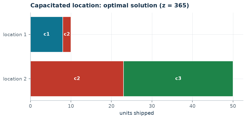
What the solver says. \(z(\mathit{LP}) = 1581/5\) exactly: the hand-built dual solution is already optimal. Strengthening with \(x_l \le 1\), \(z(\mathit{LP}^+) = 317\). \(z(\mathit{MILP}) = 365\), with both locations open: location 1 serves client 1 and part of client 2, location 2 the rest of client 2 and all of client 3. Heuristic gap \(20.3\%\).
| \(UB\) | \(LB\) (dual) | \(z(\mathit{LP})\) | \(z(\mathit{LP}^+)\) | \(z(\mathit{MILP})\) | heuristic gap |
|---|---|---|---|---|---|
| 439 | \(1581/5\) | \(1581/5\) | 317 | 365 | \(20.3\%\) |
Additional considerations
- If \(u_l < d_c\) no single location can satisfy client \(c\)'s demand alone: not the case here, but worth checking.
- \(y_{lc} \le d_c\, x_l\) is valid but implied jointly by the two constraints.
Additional modelling questions
8.1.1 — Minimum lot for every open location
Every open location must ship at least \(5\) liters. How does the model change? What is the new optimum?
A worked variant: conditional opening
Location 2 can only be installed if location 1 is also installed (say, a supervision requirement).
This is a link between two variables of the same family, imposed by the single linear constraint
(one linear constraint): if \(x_2 = 1\) then necessarily \(x_1 = 1\). On the instance the optimum of problem 8.1 already opens both locations, so the additional constraint is not binding and the optimum stays \(365\).
"Site 2 opens only if site 1 opens" adds \(\rho \le 0\) to the dual, which moves fixed cost between the two sites: \(\mu_1 = (i_1 + \rho)/u_1\) and \(\mu_2 = (i_2 - \rho)/u_2\). One tries \(\rho\) among the values that change the minimum defining \(\pi_c\); on this instance the best is \(\rho = 0\), because site 1 already has the lowest cost per litre.
| value | what it is | |
|---|---|---|
| \(\mathit{UB}\) | \(439\) | heuristic solution |
| \(\mathit{LB}\) | \(\frac{1581}{5}\) | dual certificate built by hand |
| \(z(\mathit{LP})\) | \(325\) | relaxation without the bounds |
| \(z(\mathit{LP}^+)\) | \(325\) | relaxation with the bounds |
| \(z(\mathit{MILP})\) | \(365\) | optimum of the MILP |
Code
Full script —
python/fam08_1_capacitated.py
(reproducible with python3 python/fam08_1_capacitated.py from the
python/ folder). Notebook —
notebooks/fam08_1_capacitated.ipynb
— opens in Colab from the badge at the top of the page.
Show the complete script — python/fam08_1_capacitated.py (247 lines)
"""Problem 8.1 -- Capacitated facility location (minimum cost).

Aggregated activation link between the binary variable x_l (open location l)
and the continuous flow variables y_lc: the link is proved in both
directions exactly as in problem 7.2, but here the link constraint is also a
capacity constraint (one single family of constraints does both jobs).
"""
import gurobipy as gp
import pandas as pd
from gurobipy import GRB

from mip import (ammissibile, dualita_forte, due_rilassamenti, frazione,
                 nuovo_modello, registra_bound, rilassamenti, risolvi,
                 stampa_soluzione, valuta)
from stile import CICLO, intestazione, plt, salva_dati, salva_figura
from esteso import salva_modello

R = range

# ---------- 1. MODEL AND INSTANCE ----------

intestazione("1. Capacitated facility location: where to open, how much to ship")
t1 = [[4, 5, 6], [6, 4, 3]]      # transport cost location l -> client c
u1 = [50, 50]                    # capacity of each location
i1 = [60, 90]                    # opening cost
d1 = [8, 25, 27]                 # client demand
m, n = 2, 3
salva_dati(pd.DataFrame([{"location": l + 1, "client": c + 1, "t": t1[l][c]}
                         for l in R(m) for c in R(n)]), "fam08_1_costi")
salva_dati(pd.DataFrame({"location": R(1, m + 1), "u": u1, "i": i1}), "fam08_1_sedi")
salva_dati(pd.DataFrame({"client": R(1, n + 1), "d": d1}), "fam08_1_clienti")


def modello_1(t, u, i, d):
    m, n = len(u), len(d)
    mod = nuovo_modello("capacitated_location")
    x = mod.addVars(m, vtype=GRB.BINARY, name="x")
    y = mod.addVars(m, n, name="y")
    mod.setObjective(gp.quicksum(i[l] * x[l] for l in R(m))
                      + gp.quicksum(t[l][c] * y[l, c] for l in R(m) for c in R(n)), GRB.MINIMIZE)
    mod.addConstrs((u[l] * x[l] - gp.quicksum(y[l, c] for c in R(n)) >= 0 for l in R(m)),
                   name="capacity")
    mod.addConstrs((gp.quicksum(y[l, c] for l in R(m)) == d[c] for c in R(n)), name="demand")
    return mod, x, y


def duale_1(t, u, i, d):
    """min sum d_c pi_c;  u_l mu_l <= i_l;  -mu_l + pi_c <= t_lc;  mu >= 0, pi free."""
    m, n = len(u), len(d)
    dl = nuovo_modello("duale_location")
    mu = dl.addVars(m, name="mu")
    pi = dl.addVars(n, lb=-GRB.INFINITY, name="pi")
    dl.setObjective(gp.quicksum(d[c] * pi[c] for c in R(n)), GRB.MAXIMIZE)
    dl.addConstrs((u[l] * mu[l] <= i[l] for l in R(m)), name="rc_x")
    dl.addConstrs((-mu[l] + pi[c] <= t[l][c] for l in R(m) for c in R(n)), name="rc_y")
    return dl


m1, x1, y1 = modello_1(t1, u1, i1, d1)
salva_modello(m1, "fam08_1_primale")

# ---------- 2. THE LP RELAXATION ----------
zlp1, zlp1r, _ = rilassamenti(m1)

# ---------- 3. THE DUAL OF THE RELAXATION (LOWER BOUND) ----------

d1_ = duale_1(t1, u1, i1, d1)
salva_modello(d1_, "fam08_1_duale")
mano = {f"mu[{l}]": i1[l] / u1[l] for l in R(m)}
mano.update({f"pi[{c}]": min(t1[l][c] + mano[f"mu[{l}]"] for l in R(m)) for c in R(n)})
lb1, viol = valuta(d1_, mano)
assert viol <= 1e-9, viol
print("Hand-built dual solution: mu_l = i_l/u_l = " + ", ".join(frazione(i1[l] / u1[l]) for l in R(m))
      + ";  pi_c = min_l (t_lc + mu_l) = " + ", ".join(frazione(mano[f"pi[{c}]"]) for c in R(n))
      + f"  ->  lb = {frazione(lb1)}")
dualita_forte(d1_, zlp1)

# ---------- 4. CONSTRUCTIVE HEURISTIC (UPPER BOUND) ----------

print("Heuristic: locations are scanned in order, filling each client's residual demand")
print("with each location's residual capacity, without exceeding either one.")


def euristica_1(t, u, i, d):
    m, n = len(u), len(d)
    y, x, rc, rd, passi = {}, [0] * m, list(u), list(d), []
    for l in R(m):
        for c in R(n):
            if rd[c] > 0 and rc[l] > 0:
                q = min(rd[c], rc[l])
                y[(l, c)] = q
                rd[c] -= q
                rc[l] -= q
                passi.append(f"Location {l + 1}, client {c + 1}: ship min(rd={rd[c] + q}, rc={rc[l] + q}) = {q}; "
                             f"rd[{c + 1}] = {rd[c]}, rc[{l + 1}] = {rc[l]}.")
        if rc[l] < u[l]:
            x[l] = 1
            passi.append(f"Location {l + 1} shipped something (rc = {rc[l]} < u = {u[l]}): it opens, x[{l + 1}] = 1.")
    ok = all(v == 0 for v in rd)
    return x, y, passi, ok


xe, ye, passi, ok = euristica_1(t1, u1, i1, d1)
for i, s in enumerate(passi, 1):
    print(f"  Step {i}. {s}")
assert ok, "heuristic infeasible: demand not satisfied"
ub1 = sum(i1[l] * xe[l] for l in R(m)) + sum(t1[l][c] * ye.get((l, c), 0) for l in R(m) for c in R(n))
sol_eur = {f"x[{l}]": xe[l] for l in R(m)}
sol_eur.update({f"y[{l},{c}]": v for (l, c), v in ye.items()})
assert ammissibile(m1, sol_eur)
print(f"  ub = {ub1}")

# ---------- 5. OPTIMAL SOLUTION OF THE MILP ----------

z1 = risolvi(m1)
print("Optimal solution of the MILP:")
stampa_soluzione(m1, solo_non_nulle=True)
riga = registra_bound("1 capacitated location", ub1, lb1, zlp1, zlp1r, z1)
salva_dati(pd.DataFrame([riga]), "fam08_1_bound")

# ---------- 6. ADDITIONAL MODELLING QUESTIONS ----------

varianti = {}


def variante(nome, mod):
    z = risolvi(mod)
    print(f"  {nome:70s} z = {frazione(z)}")
    return z


# 1a: every open location must ship at least 5 units (minimum lot / semi-continuous)
mod, x, y = modello_1(t1, u1, i1, d1)
mod.addConstrs((gp.quicksum(y[l, c] for c in R(n)) >= 5 * x[l] for l in R(m)), name="minimum_lot")
varianti["1a"] = variante("1a. Every open location ships at least 5 units (sum_c y_lc >= 5 x_l)", mod)
# 1b: location 2 opens only if location 1 opens
mod, x, y = modello_1(t1, u1, i1, d1)
mod.addConstr(x[1] <= x[0], name="2_only_if_1")
varianti["1b"] = variante("1b. Location 2 opens only if location 1 opens (x_2 <= x_1)", mod)
salva_dati(pd.DataFrame({"variant": list(varianti), "z": list(varianti.values())}), "fam08_1_varianti")

# ---------- 7. THE SANDWICH ON THE VARIANT 1b ----------
intestazione("1b. The sandwich on the variant: site 2 opens only if site 1 opens")


def modello_1b(t, u, i, d):
    mod_, xx, yy = modello_1(t, u, i, d)
    mod_.addConstr(xx[1] - xx[0] <= 0, name="2_solo_se_1")
    return mod_, xx, yy


def duale_1b(t, u, i, d):
    """To the dual of 8.1 one adds rho <= 0 for the constraint x_2 - x_1 <= 0: it
    loosens the column of site 1 and tightens that of site 2. The right-hand
    side is zero, so the objective does not change."""
    mm, nn = len(u), len(d)
    dl = nuovo_modello("duale_localizzazione_1b")
    mu = dl.addVars(mm, name="mu")
    pi = dl.addVars(nn, lb=-GRB.INFINITY, name="pi")
    rho = dl.addVar(lb=-GRB.INFINITY, ub=0.0, name="rho")
    dl.setObjective(gp.quicksum(d[c] * pi[c] for c in R(nn)), GRB.MAXIMIZE)
    dl.addConstr(u[0] * mu[0] - rho <= i[0], name="rc_x0")
    dl.addConstr(u[1] * mu[1] + rho <= i[1], name="rc_x1")
    dl.addConstrs((-mu[l] + pi[c] <= t[l][c] for l in R(mm) for c in R(nn)), name="rc_y")
    return dl


m1b, x1b, y1b = modello_1b(t1, u1, i1, d1)
salva_modello(m1b, "fam08_1b_primale")

# -- feasible heuristic: the base one, repaired by opening site 1 as well --
print("Constructive heuristic: start from the solution of the base problem; if it opens site 2")
print("without site 1, open site 1 too (the demand stays served, only the fixed cost changes).")
aperte = [l for l in R(m) if xe[l]]
print(f"  base solution: sites open {[l + 1 for l in aperte]}, cost {frazione(ub1)}")
aperte_b = sorted(set(aperte) | ({0} if 1 in aperte else set()))
ub1b = sum(i1[l] for l in aperte_b) + sum(t1[l][c] * ye.get((l, c), 0)
                                          for l in R(m) for c in R(n))
sol_1b = {f"x[{l}]": (1 if l in aperte_b else 0) for l in R(m)}
sol_1b.update({f"y[{l},{c}]": v for (l, c), v in ye.items()})
assert ammissibile(m1b, sol_1b), "the heuristic solution of the variant must be feasible"
print(f"  after the repair: sites {[l + 1 for l in aperte_b]}  ->  ub = {frazione(ub1b)}")

# -- dual certificate: rho moves fixed cost from site 2 to site 1 --
d1b_ = duale_1b(t1, u1, i1, d1)
salva_modello(d1b_, "fam08_1b_duale")


def valore_duale_1b(rho_val):
    mu_v = {0: (i1[0] + rho_val) / u1[0], 1: (i1[1] - rho_val) / u1[1]}
    if min(mu_v.values()) < 0:
        return None, None, None
    pi_v = {c: min(t1[l][c] + mu_v[l] for l in R(m)) for c in R(n)}
    return sum(d1[c] * pi_v[c] for c in R(n)), mu_v, pi_v


# rho is non-positive: it is tried on the grid of values that make a column
# tight, that is where the minimum defining pi_c changes site
candidati_1b = [0.0] + [-(u1[0] * (t1[1][c] + i1[1] / u1[1] - t1[0][c]) - i1[0])
                        * u1[1] / (u1[0] + u1[1]) for c in R(n)]
candidati_1b = [r for r in candidati_1b if r <= 0 and valore_duale_1b(r)[0] is not None]
scelto_1b = max(candidati_1b, key=lambda r: valore_duale_1b(r)[0])
lb1b, mu_1b, pi_1b = valore_duale_1b(scelto_1b)
mano_1b = ({f"mu[{l}]": mu_1b[l] for l in R(m)}
           | {f"pi[{c}]": pi_1b[c] for c in R(n)} | {"rho": scelto_1b})
lb1b_val, viol_1b = valuta(d1b_, mano_1b)
assert viol_1b <= 1e-9, viol_1b
print("Dual solution by hand: rho moves fixed cost from site 2 to site 1, that is")
print("  mu_1 = (i_1 + rho)/u_1 and mu_2 = (i_2 - rho)/u_2; then pi_c = min_l (t_lc + mu_l)")
print(f"  as in the base problem. rho is tried among the values that change that minimum:")
print(f"  rho = {frazione(scelto_1b)}  ->  lb = {frazione(lb1b_val)}")
if abs(scelto_1b) < 1e-9:
    print("  Here the best is rho = 0: site 1 already has the lowest cost per litre,")
    print("  and moving more fixed cost to it would lower mu_2 more than it raises mu_1.")
    print("  The certificate of the variant coincides with the one of the base problem.")
zlp1b, zlp1br, _ = due_rilassamenti(m1b, d1b_)
z1b = risolvi(m1b)
riga_1b = registra_bound("1b site 2 only with site 1", ub1b, lb1b_val, zlp1b, zlp1br, z1b)
salva_dati(pd.DataFrame([riga_1b]), "fam08_1b_bound")
assert lb1b_val <= zlp1b <= z1b <= ub1b + 1e-9

# ---------- 8. FIGURES ----------


def barre_flusso(y, m, n, titolo, nome):
    """For each location, a stacked bar of the units shipped to each client."""
    fig, ax = plt.subplots(figsize=(7.2, 3.0))
    for l in R(m):
        inizio = 0
        for c in R(n):
            q = y.get((l, c), 0)
            if q > 0:
                ax.barh(l, q, left=inizio, color=CICLO[c % len(CICLO)], edgecolor="white")
                ax.text(inizio + q / 2, l, f"c{c + 1}", ha="center", va="center", color="white",
                        fontsize=9, fontweight="bold")
                inizio += q
    ax.set_yticks(R(m))
    ax.set_yticklabels([f"location {l + 1}" for l in R(m)])
    ax.set_xlabel("units shipped")
    ax.set_title(titolo)
    ax.invert_yaxis()
    salva_figura(fig, nome)


ott_y = {(l, c): y1[l, c].X for l in R(m) for c in R(n) if y1[l, c].X > 1e-6}
barre_flusso(ott_y, m, n, f"Capacitated location: optimal solution (z = {frazione(z1)})", "cap08_capacitata_ottimo")
print("Fine.")