Production with quadratic smoothing
Lecture notes (PDF) · Chapter slides (PDF) · Exercises
Class: convex QP · Script: python/lab04_production_quadratic.py

Prerequisites
-
From the module LP Modelling, Chapter 4 «Multi-period production and inventory»: the linear production and inventory model, with its data.
-
From this module, Chapter 2 «Background: convexity, quadratic programming and KKT conditions»: convex quadratic programs, the KKT conditions and the multipliers as shadow prices.
-
From this module, Chapter 3 «The solver for nonlinear models»: quadratic objectives and the multipliers of a QP in
gurobipy.
Objectives
At the end of this chapter you will be able to:
-
add a convex quadratic term to a linear model;
-
read the multipliers of a QP and verify them by perturbation;
-
trace the cost-smoothness frontier as the weight varies.
The case, the data and the linear model are those of LP Modelling, "Production and inventory". The minimum-cost plan changes pace abruptly: total production goes from 219.5 to 389.0 units, with jumps of up to 81.4 units in a month. Here a quadratic penalty on the jumps of total production is added to the objective: a jump twice as large costs four times as much.
Model
What changes. Data, variables and constraints are those of the linear model (\(x_{it}\) production, \(s_{it}\) stock, demand \(d_{it}\), costs \(c_{it}\) and \(h_{it}\), hours \(a_i\), capacity \(b_t\)). A single datum is added:
| Symbol | Type | Meaning |
|---|---|---|
| \(\gamma\) | \(\in \mathbb{Q}_{\ge 0}\) | weight of the jumps of total production (€ per unit²) |
Using the same variables, a QP model for the problem is the following:
Description of the objective function and of the constraints:
- the quadratic objective function adds to the production and holding cost the weight \(\gamma\) times the square of every jump of total production;
- the linear balance constraints of the inventory (\(n\,m\) linear constraints);
- the linear capacity constraints (\(m\) linear constraints);
- the non-negativity constraints define the variables of the model.
The QP is convex: every jump is linear in the variables, its square is convex and the constraints are linear. With \(\gamma = 0\) we recover the linear model.
Worked example (1 product, 2 months)
\(d = (60, 100)\), \(c = 10\), \(h = 1\), ample capacity; the linear model produces to demand, cost \(1600\). With \(\gamma = 0.5\) the solver gives \(\tilde x = (79.75;\ 80.25)\), \(\tilde s_1 = 19.75\), \(\tilde z = 1619.875\) and balance multipliers \((9.5;\ 10.5)\). From the balances the jump is \(40 - 2s_1\) and the objective \(f(s_1) = 1600 + s_1 + \gamma(40 - 2s_1)^2\): \(f'(s_1) = 0\) gives \(s_1 = 20 - 1/(8\gamma)\). For \(\gamma \le 1/160\) it pays to keep no stock. With positive stock the KKT conditions give \(\tilde\pi_2 - \tilde\pi_1 = h\).
Results
gamma = 0.0: objective 32,889.33  linear cost 32,889.33  largest jump 81.4
   total production:  219.5  301.0  341.4  374.3  389.0  324.8
gamma = 0.5: objective 33,003.10  linear cost 33,000.96  largest jump  1.2
   total production:  323.3  324.3  325.5  326.1  325.9  324.8
gamma = 2.0: objective 33,004.74  linear cost 33,004.14  largest jump  0.4
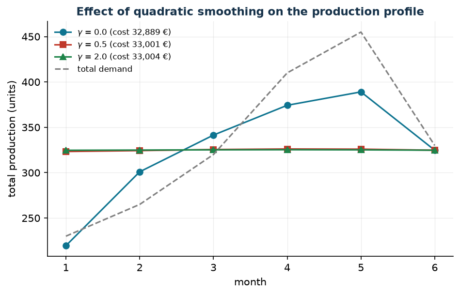
The smooth plan costs €111.63 more than the linear plan (+0.34%). Mostly product 1 goes to stock, up to 212.6 units: the penalty counts units, not hours, and product 1 gives more units per machine hour (\(a_1 = 0.9\)). In the linear model the stock built in advance was that of product 3.
Sensitivity
month 4: Pi(gamma=0) = -2.286   Pi(gamma=0.5) = -0.667 EUR/hour
month 5: Pi(gamma=0) = -3.048   Pi(gamma=0.5) = -1.333 EUR/hour
month 6: Pi(gamma=0) = -3.810   Pi(gamma=0.5) = -3.134 EUR/hour
Check: +1    hour  in month 6 -> difference quotient -3.060
Check: +0.01 hours in month 6 -> difference quotient -3.133
The multiplier of a QP is exact only at the margin
In the QP the optimal value has curvature: with a whole hour the change is \(-3.060\), with \(0.01\) hours the difference quotient is \(-3.133\), that is the multiplier. With smoothing the capacity of months 1–3 is no longer active.
Management take-away
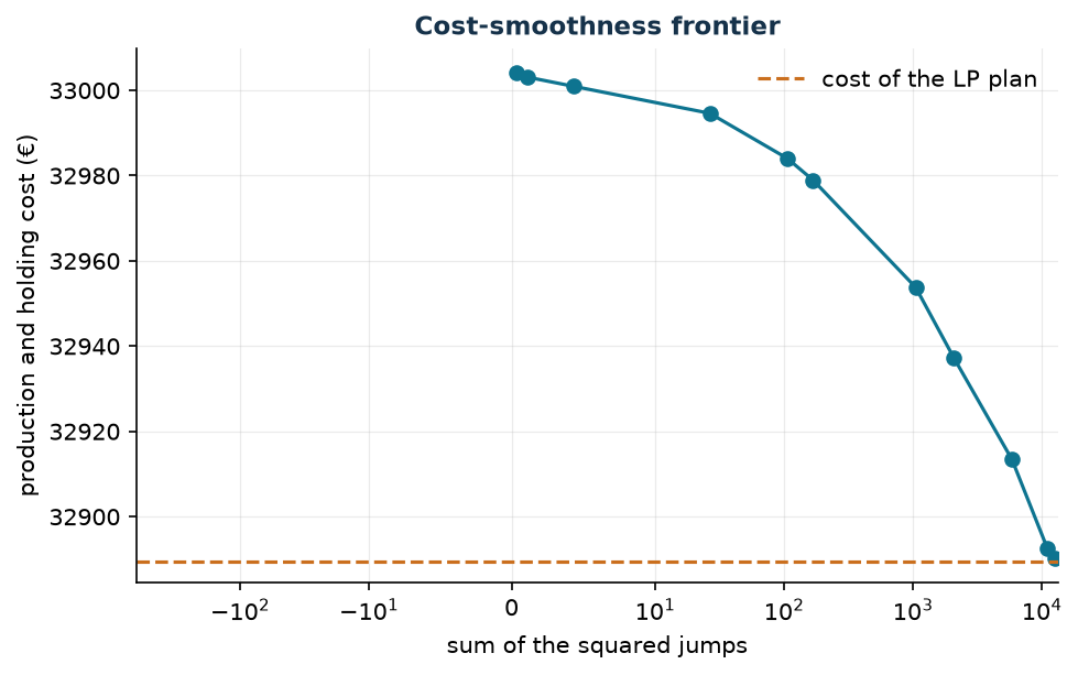
The first steps towards smoothness cost very little: with \(\gamma = 0.01\) the sum of the squared jumps falls from 13,699 to 2,075 for €48. An almost flat plan costs about €112 out of 33,000.
In summary
In summary
-
A convex quadratic term added to an LP gives a convex QP.
-
The weight \(\gamma\) traces the cost-smoothness frontier: the first steps cost little.
-
QP multipliers are read with
Pi, but they hold at the margin. -
A new term can change the structure of the solution.
Code
The full script of the chapter is
python/lab04_production_quadratic.py
(reproducible with python3 lab04_production_quadratic.py from the python/ folder);
the same code is in the notebook that opens in Colab from the badge at the top of the
page.
Show the full script — lab04_production_quadratic.py
"""Chapter 4 — Production with quadratic smoothing (convex QP).

Case study: the same as the linear production and inventory model
(LP Modelling): 3 components (products 1, 2, 3), 6 months, one shared
resource (machine hours). Here a quadratic penalty on the month-to-month
changes of total production is added to the objective.

Contents:
  1. Data (the same as in the linear case)
  2. Worked example: one product, two months
  3. The QP on the case study for three values of gamma
  4. Capacity multipliers in the QP and check by perturbation
  5. Sensitivity: the cost-smoothness frontier as gamma varies
"""
import gurobipy as gp
import numpy as np
import pandas as pd
from gurobipy import GRB

from stile import ARANCIO, TEAL, intestazione, plt, salva_dat, salva_dati, salva_figura

# ----------------------------------------------------------------------
# 1. DATA (the same as in the linear case)
# ----------------------------------------------------------------------
# The data are those of the linear case in LP Modelling: they are written here (same seed),
# so that the script also runs in Colab; the CSV files live in the LP Modelling repository.
prodotti = ["1", "2", "3"]
mesi = list(range(1, 7))
domanda = {
    ("1", 1): 110, ("1", 2): 130, ("1", 3): 150, ("1", 4): 190, ("1", 5): 210, ("1", 6): 160,
    ("2", 1): 70,  ("2", 2): 80,  ("2", 3): 110, ("2", 4): 140, ("2", 5): 150, ("2", 6): 100,
    ("3", 1): 50,  ("3", 2): 55,  ("3", 3): 60,  ("3", 4): 80,  ("3", 5): 95,  ("3", 6): 70,
}
costo_prod = {"1": 12.0, "2": 18.0, "3": 25.0}   # €/unit
costo_giac = {"1": 0.8, "2": 1.2, "3": 1.6}      # €/unit/month
ore_unit = {"1": 0.9, "2": 1.4, "3": 2.1}        # machine hours per unit
capacita = {1: 420, 2: 420, 3: 460, 4: 460, 5: 460, 6: 420}  # hours/month
scorta_iniziale = {"1": 30, "2": 20, "3": 10}


def costruisci_qp(gamma, cap=None):
    """QP: production + holding cost + gamma * sum of the squared jumps."""
    cap = cap or capacita
    m = gp.Model("production_smoothing")
    m.Params.OutputFlag = 0
    x = m.addVars(prodotti, mesi, name="x")           # quantity produced
    s = m.addVars(prodotti, mesi, name="s")           # end-of-month stock
    m.addConstrs(
        ((scorta_iniziale[i] if t == 1 else s[i, t - 1]) + x[i, t] == domanda[i, t] + s[i, t]
         for i in prodotti for t in mesi), name="balance")
    v_cap = m.addConstrs(
        (gp.quicksum(ore_unit[i] * x[i, t] for i in prodotti) <= cap[t] for t in mesi),
        name="capacity")
    tot = {t: gp.quicksum(x[i, t] for i in prodotti) for t in mesi}
    costo = gp.quicksum(costo_prod[i] * x[i, t] + costo_giac[i] * s[i, t]
                        for i in prodotti for t in mesi)
    salti = gp.quicksum((tot[t] - tot[t - 1]) * (tot[t] - tot[t - 1]) for t in mesi[1:])
    m.setObjective(costo + gamma * salti, GRB.MINIMIZE)
    return m, x, s, v_cap


def leggi(m, x, s):
    """Linear cost, total profile, jumps and sum of the squared jumps."""
    profilo = np.array([sum(x[i, t].X for i in prodotti) for t in mesi])
    salti = np.diff(profilo)
    costo = sum(costo_prod[i] * x[i, t].X + costo_giac[i] * s[i, t].X
                for i in prodotti for t in mesi)
    return costo, profilo, salti, float((salti ** 2).sum())


# ----------------------------------------------------------------------
# 2. WORKED EXAMPLE: ONE PRODUCT, TWO MONTHS
# ----------------------------------------------------------------------
intestazione("Worked example: one product, two months (d = 60, 100; c = 10, h = 1)")
for g in (0.0, 0.004, 0.5):
    me = gp.Model("example")
    me.Params.OutputFlag = 0
    x1, x2, s1 = me.addVar(name="x1"), me.addVar(name="x2"), me.addVar(name="s1")
    b1 = me.addConstr(x1 == 60 + s1, name="bal1")
    b2 = me.addConstr(s1 + x2 == 100, name="bal2")
    me.setObjective(10 * x1 + 10 * x2 + s1 + g * (x2 - x1) * (x2 - x1), GRB.MINIMIZE)
    me.optimize()
    print(f"  gamma = {g:5.3f}: x1 = {x1.X:7.3f}  x2 = {x2.X:7.3f}  s1 = {s1.X:6.3f}  "
          f"cost = {me.ObjVal:9.4f}  Pi = ({b1.Pi:.4f}, {b2.Pi:.4f})")
print(f"  threshold: s1 > 0 only if gamma > 1/160 = {1 / 160:.5f}; "
      f"with gamma = 0.5: s1 = 20 - 1/(8 gamma) = {20 - 1 / (8 * 0.5):.2f}")

# ----------------------------------------------------------------------
# 3. THE QP ON THE CASE STUDY
# ----------------------------------------------------------------------
intestazione("QP on the case study: three values of gamma")
GAMMA = [0.0, 0.5, 2.0]
risultati = {}
for g in GAMMA:
    m, x, s, v_cap = costruisci_qp(g)
    m.optimize()
    assert m.Status == GRB.OPTIMAL
    costo, profilo, salti, sq = leggi(m, x, s)
    risultati[g] = dict(obj=m.ObjVal, costo=costo, profilo=profilo, salti=salti, sq=sq,
                        piano={(i, t): x[i, t].X for i in prodotti for t in mesi},
                        scorte={(i, t): s[i, t].X for i in prodotti for t in mesi},
                        pi=[v_cap[t].Pi for t in mesi])
    print(f"gamma = {g:3.1f}: objective {m.ObjVal:10.2f} €  linear cost {costo:10.2f} €  "
          f"largest jump {np.abs(salti).max():6.1f}  sum of jumps^2 {sq:9.1f}")
    print("   total production: " + "  ".join(f"{v:6.1f}" for v in profilo))

r5 = risultati[0.5]
print(f"\nCost of smoothness (gamma = 0.5): {r5['costo'] - risultati[0.0]['costo']:.2f} € "
      f"(+{100 * (r5['costo'] / risultati[0.0]['costo'] - 1):.2f}%)")
print("\nPlan with gamma = 0.5 (units/month):")
piano5 = pd.DataFrame([(i, t, r5["piano"][i, t], r5["scorte"][i, t]) for i in prodotti for t in mesi],
                      columns=["product", "month", "production", "stock"])
print(piano5.pivot(index="product", columns="month", values="production").round(1))
print("End-of-month stocks:")
print(piano5.pivot(index="product", columns="month", values="stock").round(1))
salva_dati(piano5, "produzione_piano_regolare")

# ----------------------------------------------------------------------
# 4. CAPACITY MULTIPLIERS IN THE QP
# ----------------------------------------------------------------------
intestazione("Capacity multipliers (gamma = 0 and gamma = 0.5)")
for t in mesi:
    print(f"  month {t}: Pi(gamma=0) = {risultati[0.0]['pi'][t - 1]:7.3f}   "
          f"Pi(gamma=0.5) = {r5['pi'][t - 1]:7.3f} €/hour")
t_star = int(np.argmin(r5["pi"])) + 1
for eps in (1.0, 0.01):
    cap2 = dict(capacita)
    cap2[t_star] += eps
    m2, x2_, s2_, _ = costruisci_qp(0.5, cap2)
    m2.optimize()
    print(f"Check: +{eps:g} hours in month {t_star} -> objective from {r5['obj']:.3f} to {m2.ObjVal:.3f} "
          f"(difference quotient {(m2.ObjVal - r5['obj']) / eps:+.3f}; Pi = {r5['pi'][t_star - 1]:.3f})")

# ----------------------------------------------------------------------
# 5. SENSITIVITY: COST-SMOOTHNESS FRONTIER
# ----------------------------------------------------------------------
intestazione("Cost-smoothness frontier as gamma varies")
griglia = [0.0, 0.001, 0.002, 0.005, 0.01, 0.02, 0.05, 0.1, 0.2, 0.5, 1.0, 2.0]
frontiera = []
for g in griglia:
    m, x, s, _ = costruisci_qp(g)
    m.optimize()
    costo, profilo, salti, sq = leggi(m, x, s)
    frontiera.append((g, costo, sq, float(np.abs(salti).max())))
    print(f"  gamma = {g:6.3f}: cost {costo:10.2f} €  sum of jumps^2 {sq:9.1f}  "
          f"largest jump {np.abs(salti).max():6.1f}")
front = pd.DataFrame(frontiera, columns=["gamma", "cost", "squared_jumps", "largest_jump"])
salva_dati(front, "produzione_frontiera_regolarita")

# ----------------------------------------------------------------------
# 6. FIGURES (data for pgfplots + matplotlib preview)
# ----------------------------------------------------------------------
salva_dat(pd.DataFrame({
    "mese": mesi,
    "gzero": risultati[0.0]["profilo"], "gmezzo": risultati[0.5]["profilo"],
    "gdue": risultati[2.0]["profilo"],
    "domtot": [sum(domanda[i, t] for i in prodotti) for t in mesi],
}), "cap04_smoothing")
salva_dat(front[front["gamma"] > 0], "cap04_frontiera")

fig, ax = plt.subplots()
for g, st in zip(GAMMA, ["-o", "-s", "-^"]):
    ax.plot(mesi, risultati[g]["profilo"], st,
            label=f"$\\gamma$ = {g} (cost {risultati[g]['costo']:,.0f} €)")
ax.plot(mesi, [sum(domanda[i, t] for i in prodotti) for t in mesi], "--", color="gray",
        label="total demand")
ax.set_xlabel("month"); ax.set_ylabel("total production (units)")
ax.set_title("Effect of quadratic smoothing on the production profile")
ax.legend(fontsize=8)
salva_figura(fig, "cap04_smoothing")

fig, ax = plt.subplots()
f2 = front[front["gamma"] > 0]
ax.plot(f2["squared_jumps"], f2["cost"], "-o", color=TEAL)
ax.axhline(risultati[0.0]["costo"], color=ARANCIO, ls="--", label="cost of the LP plan")
ax.set_xscale("symlog", linthresh=10)
ax.set_xlabel("sum of the squared jumps")
ax.set_ylabel("production and holding cost (€)")
ax.set_title("Cost-smoothness frontier")
ax.legend()
salva_figura(fig, "cap04_frontiera")

print("\nDone: chapter 4.")
Exercises
- By hand — in the example set \(\gamma = 0.05\): compute \(s_1\), \(x_1\), \(x_2\), the optimal value and the balance multipliers.
- Check — with \(\gamma = 0.5\) verify by perturbation the capacity multiplier of month 5 (increments of 1 and of 0.01 hours) and compare with month 6.
- Smoothing by product — penalize the jumps of every product, \(\gamma \sum_i \sum_t (x_{it} - x_{i,t-1})^2\), with \(\gamma = 0.5\).
- Linear smoothing — replace the square with the absolute value (an LP), with \(\gamma = 5\): what shape does the profile take?
- Target level — penalize \(\gamma \sum_t (v_t - 325)^2\) with \(\gamma = 0.5\).